[의학통계방법론] Ch17. Simple Linear Regression

12 May 2022 in Study log / Study / 의학통계방법론 on R, Sas, Blog, Jekyll, Jupyter, Data, Python

Simple Linear Regression
R 프로그램 결과
- 17장
SAS 프로그램 결과
- 17장

Simple Linear Regression

R 프로그램 결과

R 접기/펼치기 버튼

패키지

설치된 패키지 접기/펼치기 버튼

getwd()

## [1] "C:/Biostat"

library("dplyr")
library("kableExtra")
library("ggplot2")
library("chemCal")
library("broom")

17장

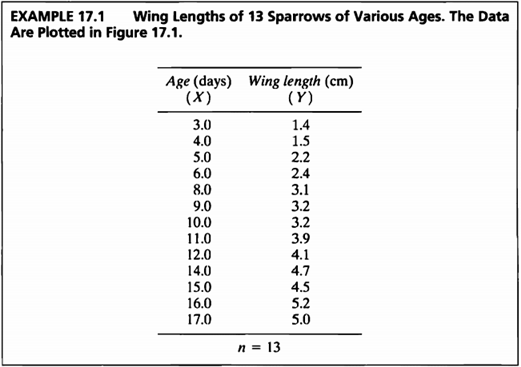
EXAMPLE 17.1

#데이터셋
age <- c(3.0,4.0,5.0,6.0,8.0,9.0,10.0,11.0,12.0,14.0,15.0,16.0,17.0)
wing_length<-c(1.4,1.5,2.2,2.4,3.1,3.2,3.2,3.9,4.1,4.7,4.5,5.2,5.0)
ex17_1 <- data.frame(age,wing_length)
ex17_1 %>%
  kbl(caption = "Dataset of Example 17.1") %>%
  kable_styling(bootstrap_options = c("striped", "hover", "condensed", "responsive"))

Dataset of Example 17.1
age	wing_length
3	1.4
4	1.5
5	2.2
6	2.4
8	3.1
9	3.2
10	3.2
11	3.9
12	4.1
14	4.7
15	4.5
16	5.2
17	5.0

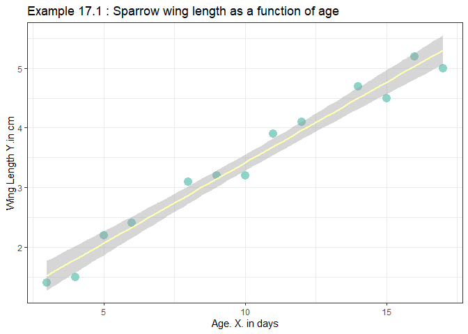
해당 데이터는 참새의 나이와 날개의 길이를 측정한 데이터이다.
이 데이터를 사용하여 연령과 날개 길이의 회귀직선을 그려보도록 한다.

library("ggplot2")
ggplot(ex17_1, aes(x=age, y=wing_length)) + 
  geom_point(color="#8dd3c7",size=4) + 
  stat_smooth(method = 'lm', color="#ffffb3")+
  ggtitle("Example 17.1 : Sparrow wing length as a function of age")+
  ylab("Wing Length Y.in cm")+
  xlab("Age. X. in days")+
  theme_bw()

EXAMPLE 17.2

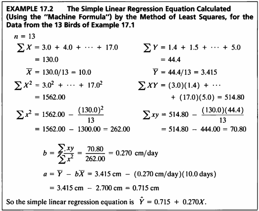
EXAMPLE 17.1 데이터로 Machine formula를 사용하여 회귀식을 구하도록 한다.

\[\begin{aligned} n&=13 \ \ \ \ \ \ \ \ \ \overline X=\frac{130}{10}=13 \ \ \ \ \ \overline Y=\frac{44.4}{10}=3.415\\ \\ \sum x^2 &= \sum X^2 - \frac{(\sum X)^2}{n} = 1562-\frac{130^2}{13}=262\\ \\ \sum xy&= \sum XY - \frac{\sum X \ * \sum Y }{n}=514.80-\frac{130*44}{13}=70.8\\ \\ b &= \frac{\sum xy}{\sum x^2}= \frac{70.8}{262}=0.270\ cm/day \\ \\ a &= \overline Y - b \overline X=3.415\ cm-(0.270\ cm/day)(10\ days)\\ \\ &= 3.415\ cm-2.7\ cm=0.715\ cm\\ \\ \therefore \hat Y &= 0.715+0.270X \end{aligned}\]

f_17_2 <- function(x){
  n <- nrow(x)
  sum_x <- sum(x[,1])
  mean_x <- mean(x[,1])
  sum_y <- sum(x[,2])
  mean_y <- mean(x[,2])
  sum_x2 <- sum(x[,1]^2)
  sum_xy <- sum(x[,1]*x[,2])
  b <- (sum_xy-((sum_x*sum_y)/n))/(sum_x2-(sum_x^2)/n)
  a <- mean_y - b*mean_x
  out <- data.frame(n,sum_x,mean_x,sum_y,mean_y,sum_x2,sum_xy,b,a)
  return(out)
}

f_17_2(ex17_1)%>%
  kbl(caption = "Result of simple linear regression equation",escape=F) %>%
  kable_styling(bootstrap_options = c("striped", "hover", "condensed", "responsive"))

Result of simple linear regression equation
n	sum_x	mean_x	sum_y	mean_y	sum_x2	sum_xy	b	a
13	130	10	44.4	3.415385	1562	514.8	0.270229	0.7130945

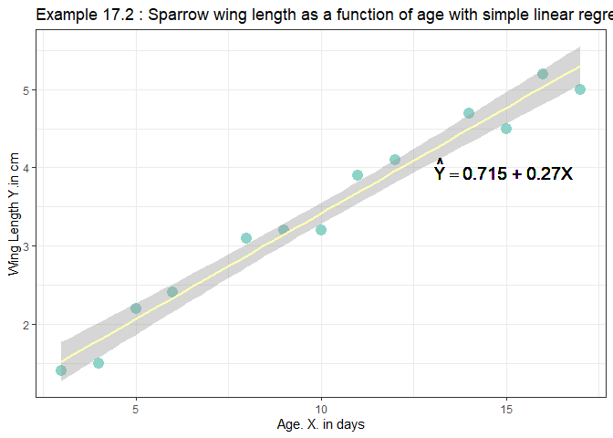
회귀식을 추정한 결과 \(\hat Y = 0.715+0.270X\) 로 도출되었다.
Example 17.1에서 구한 회귀직선에 식을 넣으면 다음과 같다.

ggplot(ex17_1, aes(x=age, y=wing_length)) + 
  geom_point(color="#8dd3c7",size=4) + 
  stat_smooth(method = 'lm', color="#ffffb3")+
  ggtitle("Example 17.2 : Sparrow wing length as a function of age with simple linear regression equation")+
  ylab("Wing Length Y.in cm")+
  xlab("Age. X. in days")+
  theme_bw()+
  geom_text(x=15, y=4, label=expression(hat(Y) == paste(0.715," + ",0.270,X, " ",)), cex = 5) 

EXAMPLE 17.3

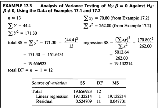
앞서 구한 회귀식의 ANOVA table을 작성하여 추정한 회귀식의 유의성을 판단하여 보겠다.

library("broom")
lm17_2 <- lm(wing_length~age,data=ex17_1)
aov17_2 <- anova(lm17_2)
aov17_2 %>% tidy() %>% 
  rename(" "="term","Sum Sq"="sumsq","Mean Sq"="meansq","F value"="statistic","Pr(>F)"="p.value") %>% 
  kable(caption = "ANOVA table",booktabs = TRUE, valign = 't') %>%
  kable_styling(bootstrap_options = c("striped", "hover", "condensed", "responsive"))

ANOVA table
	df	Sum Sq	Mean Sq	F value	Pr(\>F)
age	1	19.1322137	19.1322137	401.0875	0
Residuals	11	0.5247093	0.0477008	NA	NA

summ <- summary(lm17_2)
data.frame(summ$r.squared,summ$adj.r.squared) %>% 
  rename("R square"="summ.r.squared","Adjusted R square"="summ.adj.r.squared") %>% 
  kable(caption = "R square",booktabs = TRUE, valign = 't') %>%
  kable_styling(bootstrap_options = c("striped", "hover", "condensed", "responsive"))

R square
R square	Adjusted R square
0.9733066	0.97088

\[\begin{aligned} H_0 &: Regression\ model\ is\ not\ significant \\ H_A &: Regression\ model\ is\ significant \end{aligned}\]

회귀직선의 유의성을 판단한 결과, F값은 401.09, p-value<0.001 이므로 \(H_0: \beta_1=0\)은 기각되었다.
따라서 유의수준 5%하에 회귀직선은 유의하다고 할 수 있다.
결정계수 값은 0.97로, 총변동중에서 회귀직선에 의해 설명되는 부분이 97%임을 확인하였다.

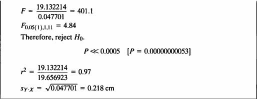
EXAMPLE 17.4

EXAMPLE 1,2에 사용된 데이터를 가지고 회귀계수의 유의성 검정을 하기 위해 t-test를 진행해 보도록 하겠다.

직접 함수를를 작성하여 구하여 보겠다.

f_17_4 <- function(x){
  alpha <- 0.05
  n <- nrow(x)
  estimate <- f_17_2(x)$b
  r2 <- summ$r.squared
  syx2 <- (sd(x[,2])*sqrt((1-r2)*(13-1)/(13-2)))^2
  sum_x2 <- sum(x[,1]^2)-(sum(x[,1])^2)/n
  se <- sqrt(syx2/sum_x2)
  t <- estimate/se
  crit <- qt(1-alpha/2,n-2)
  pvalue <- pt(t,n-2,lower.tail = F)
  if(pvalue < 0.05){
    Reject_H0 <- "yes"
  }else{
    Reject_H0 <- "No"
  }
  out <- data.frame(n,estimate,se,t,pvalue,Reject_H0)
  return(out)
}

f_17_4(ex17_1)%>%
  kbl(caption = "Result of t test",escape=F) %>%
  kable_styling(bootstrap_options = c("striped", "hover", "condensed", "responsive"))

Result of t test
n	estimate	se	t	pvalue	Reject_H0
13	0.270229	0.0134931	20.02717	0	yes

R에 내장된 함수로 구하여 보겠다.

summ$coefficients %>% 
  as.data.frame() %>% 
  kable(caption = "Coefficient",booktabs = TRUE, valign = 't') %>%
  kable_styling(bootstrap_options = c("striped", "hover", "condensed", "responsive"))

Coefficient
	Estimate	Std. Error	t value	Pr(\>\\|t\\|)
(Intercept)	0.7130945	0.1479045	4.821319	0.0005347
age	0.2702290	0.0134931	20.027169	0.0000000

본 검정의 가설은 다음과 같다.

\[\begin{aligned} H_0 &: \beta=0 \\ H_A &: \beta \ne 0 \end{aligned}\]

회귀계수의 유의성 검정 결과 age에 대한 coefficient 값은 0.2702290, t 값은 20.02 이며 p-value<0.001 로써 유의수준 0.05보다 작아 귀무가설을 기각할 충분한 근거를 가진다.
-그러므로 유의수준 5%하에 회귀계수는 유의하다고 할 수 있다.

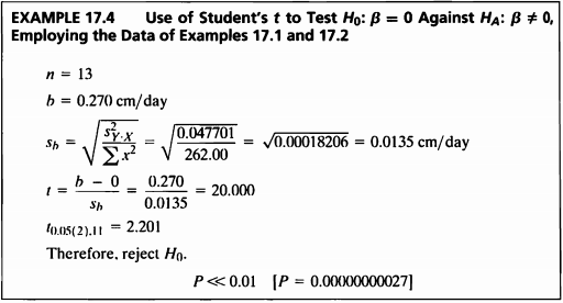
EXAMPLE 17.5

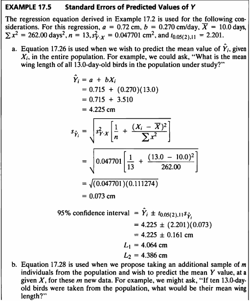
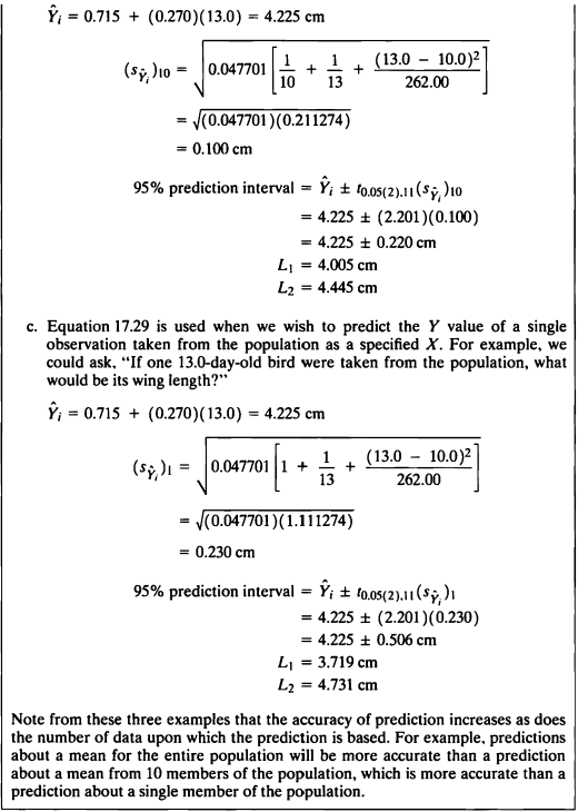
다음의 식을 통하여 표준오차를 구해해 신뢰구간을 예측해보도록 하겠겠다.

\[\begin{aligned} &n=13\\ &\hat Y_i=a+bX_+i=0.715+(0.270)(13)=422.5\ cm\\ \\ &a)\ s_{\hat Y_i} = \sqrt{s^2_{Y * X }(\frac{1}{n}+\frac{(X_i-\overline X)^2}{\sum x^2})}\\ \\ &b)\ (s_{\hat Y_i})_{m} =\sqrt{s^2_{Y * X }(\frac{1}{m}+\frac{1}{n}+\frac{(X_i-\overline X)^2}{\sum x^2})}\\ \\ &c)\ (s_{\hat Y_i})_{1} =\sqrt{s^2_{Y * X }(1+\frac{1}{n}+\frac{(X_i-\overline X)^2}{\sum x^2})} \end{aligned}\]

13 day old의 새들의 날개의 길이의 모평균은 얼마인지 표준오차를 구해 신뢰구간을 계산해보도록 하겠다.

f_17_5 <- function(x,param){
  alpha <- 0.05
  n <- nrow(x)
  b <- f_17_2(x)$b
  a <- f_17_2(x)$a
  yi <- a+b*param
  r2 <- summ$r.squared
  mean_x <- mean(x[,1])
  syx2 <- (sd(x[,2])*sqrt((1-r2)*(13-1)/(13-2)))^2
  sum_x <- sum(x[,1])
  sum_x2 <- sum(x[,1]^2)
  sumx2 <- sum_x2-(sum_x^2)/n
  syi <- sqrt(syx2*((1/param)+((param-mean_x)^2/(sum_x2-(sum_x^2)/n))))
  syi_10 <- sqrt(syx2*((1/10)+(1/param)+((param-mean_x)^2/(sum_x2-(sum_x^2)/n))))
  syi_1 <- sqrt(syx2*(1+(1/param)+((param-mean_x)^2/(sum_x2-(sum_x^2)/n))))
  crit <- qt(1-alpha/2,n-2)
  L1_1 <- yi-crit*syi
  L2_1 <- yi+crit*syi
  L1_2 <- yi-crit*syi_10
  L2_2 <- yi+crit*syi_10
  L1_3 <- yi-crit*syi_1
  L2_3 <- yi+crit*syi_1
  out <- data.frame(yi,syi,L1_1,L2_1,syi_10,L1_2,L2_2,syi_1,L1_3,L2_3)
  return(out)
}

f_17_5(ex17_1,13)%>%
  kbl(caption = "Result",escape=F) %>%
  kable_styling(bootstrap_options = c("striped", "hover", "condensed", "responsive"))

Result
yi	syi	L1_1	L2_1	syi_10	L1_2	L2_2	syi_1	L1_3	L2_3
4.226072	0.0728552	4.065719	4.386425	0.100389	4.005117	4.447026	0.2302362	3.719325	4.732818

Equation a)를 사용하였을 때 13일 살의 새의 날개 길이의 모평균의 95% 신뢰구간은 [4.065, 4.386] 이며,
b)를 사용했을 떄는 [4.005, 4.445] 그리고,
c)를 사용했을 때는 [3.719, 4.731]이다.

EXAMPLE 17.6

Estimated Y Value에 대하여 검정을 진행하여 보겠겠다.

\[\begin{aligned} H_0 &: The \ mean \ population \ wing \ length \ of \ 13.0-day-birds \ is \ not \ greater \ than \ 4cm \\ H_A &: The \ mean \ population \ wing \ length \ of \ 13.0-day-birds \ is \ greater \ than \ 4cm \end{aligned}\]

f_17_6 <- function(x,param,compare){
  alpha <- 0.05
  n <- nrow(x)
  b <- f_17_2(x)$b
  a <- f_17_2(x)$a
  yi <- a+b*param
  r2 <- summ$r.squared
  mean_x <- mean(x[,1])
  syx2 <- (sd(x[,2])*sqrt((1-r2)*(13-1)/(13-2)))^2
  sum_x <- sum(x[,1])
  sum_x2 <- sum(x[,1]^2)
  sumx2 <- sum_x2-(sum_x^2)/n
  syi <- sqrt(syx2*((1/param)+((param-mean_x)^2/(sum_x2-(sum_x^2)/n))))
  t <- (yi-compare)/syi
  crit <- qt(1-alpha/2,n-2)
  pvalue <- pt(t,n-2,lower.tail = F)
  if(pvalue < 0.05){
    Reject_H0 <- "yes"
  }else{
    Reject_H0 <- "No"
  }
  out <- data.frame(yi,t,crit,pvalue,Reject_H0)
  return(out)
}

f_17_6(ex17_1,param=13,compare=4)%>%
  kbl(caption = "Result",escape=F) %>%
  kable_styling(bootstrap_options = c("striped", "hover", "condensed", "responsive"))

Result
yi	t	crit	pvalue	Reject_H0
4.226072	3.103028	2.200985	0.0050248	yes

예측된 Y값 검정 결과 검정통계량 t값은 3.10이고 p-value=0.005 이므므로 유의수준 0.05보다 작아 귀무가설을 기각할 충분한 근거가 있다.
그러므로 유의수준5%하에 새들의 날개의 길이에 대한 모평균이 4cm 보다 크다는 충분한 근거가 있다고 할 수 있다.

EXAMPLE 17.7

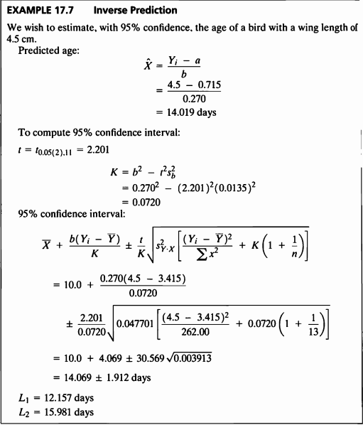
이번에는 y값이 주어졌을 때 x값을 구해보도록 하겠다.
즉, 날개의 길이가 주어졌을 때, 새들의 나이를 예측해보는 inverse에 관한 문제이다.
날개의 길이가 4.5cm 라고 했을 때 신뢰구간을 구하는 방식은 다음과 같다.

\[\begin{aligned} &\overline X + \frac{b(Y_i - \overline Y)}{K} \pm \frac{t}{K}\sqrt{(s^2_{Y*X})'[\frac{(Y_i-\overline Y)^2}{\sum x^2}+K(\frac{1}{m}+\frac{1}{n})]}\\ \\ &where\ \ t=t_{\alpha(2),(n+m-3)}, \ \ \ K=b^2-t^2(s_b^2)'\\ \\ &(s_b^2)'=\frac{(s_{Y*X}^2)'}{\sum x^2}, \ \ \ \ \ (s_{Y*X}^2)'=residual\ SS+\sum_{j=1}^m (Y_{ij}-\overline Y_i)^2/(n+m-3) \end{aligned}\]

R의 chemCal 패키지의 inverse.predict() 함수를 사용하여 구해보겠다.

library("chemCal")
inverse_result <- inverse.predict(lm17_2,4.5)
inverse_result <- as.data.frame(inverse_result)
inverse_result[2,1:3] <- "."
inverse_result %>%
  kbl(caption = "Result of Inverse Prediction",escape=F) %>%
  kable_styling(bootstrap_options = c("striped", "hover", "condensed", "responsive"))

Result of Inverse Prediction
Prediction	Standard.Error	Confidence	Confidence.Limits
14.0136897001304	0.862343975232319	1.89800629238076	12.11568
.	.	.	15.91170

위의 결과를 보아 날개의 길이가 4.5cm라고 주어졌을 때,
예상되는 새의 나이의 값은 14.013이고,
이에 대한 95% 신뢰구간은 [12.115, 15.911] 이다.

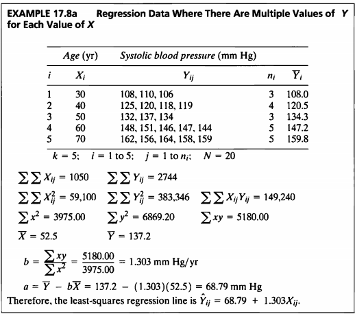
EXAMPLE 17.8a

#데이터셋
age<-c(rep(30,3),rep(40,4),rep(50,3),rep(60,5),rep(70,5))
sbp<-c(108,110,106,125,120,118,119,132,137,134,148,151,146,147,144,162,156,164,158,159)
ex17_8 <- data.frame(age,sbp)
ex17_8 %>%
  kbl(caption = "Dataset of Example 17_8a",escape=F) %>%
  kable_styling(bootstrap_options = c("striped", "hover", "condensed", "responsive"))

Dataset of Example 17_8a
age	sbp
30	108
30	110
30	106
40	125
40	120
40	118
40	119
50	132
50	137
50	134
60	148
60	151
60	146
60	147
60	144
70	162
70	156
70	164
70	158
70	159

해당 데이터는 나이와 이에 따른 수축기혈압의 데이터이다.
각각의 x에 대해 multiple value Y를 가지는 회귀분석에 대한 문제이다.

모형의 유의성 검정

\[\begin{aligned} H_0 &: Regression\ model\ is\ not\ significant \\ H_A &: Regression\ model\ is\ significant \end{aligned}\]

lm17_8 <- lm(sbp~age,data=ex17_8)
aov17_8 <- anova(lm17_8)
aov17_8%>% tidy() %>% 
  rename(" "="term","Sum Sq"="sumsq","Mean Sq"="meansq","F value"="statistic","Pr(>F)"="p.value") %>% 
  kable(caption = "ANOVA table",booktabs = TRUE, valign = 't') %>%
  kable_styling(bootstrap_options = c("striped", "hover", "condensed", "responsive"))

ANOVA table
	df	Sum Sq	Mean Sq	F value	Pr(\>F)
age	1	6750.2893	6750.289308	1021.819	0
Residuals	18	118.9107	6.606149	NA	NA

모형의 유의성 검정 결과 검정통계량 F값은 1021.819, p-value<0.001이므로 유의수준 0.05보다 작아 귀무가설을 기각할 충분한 근거를 가진다.
그러므로 유의수준 5%하에 회귀모형은 유의하다고 할 수 있다.

회귀계수의 유의성 검정

\[\begin{aligned} H_0 &: \beta=0 \\ H_A &: \beta \ne 0 \end{aligned}\]

summary(lm17_8)[4] %>% 
  as.data.frame %>% 
  rename("Estimate"="coefficients.Estimate","Standard Error"="coefficients.Std..Error","t value"="coefficients.t.value","Pr(>F)"="coefficients.Pr...t..") %>% 
  kable(caption = "Test of Coefficients",booktabs = TRUE, valign = 't') %>%
  kable_styling(bootstrap_options = c("striped", "hover", "condensed", "responsive"))

Test of Coefficients
	Estimate	Standard Error	t value	Pr(\>F)
(Intercept)	68.784906	2.2160746	31.03907	0
age	1.303145	0.0407667	31.96590	0

회귀계수의 유의성 검정 결과 검정통계량 t값은 31.039, p-value<0.001이므로 유의수준 0.05보다 작아 귀무가설을 기각할 충분한 근거를 갖는다.
그러므로 유의수준 5%하에 회귀계수는 유의하다고 할 수 있다.
추정된 회귀식은 \(\hat Y_{ij}=68.78+1.303X_{ij}\) 이다.
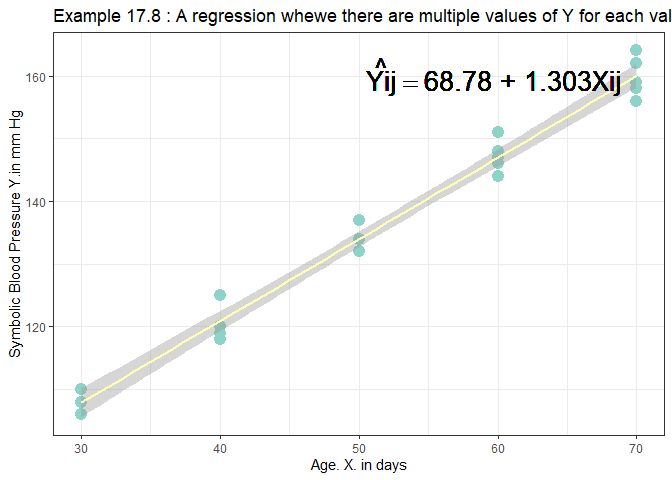
회귀선을 그려보면 다음과 같다.

ggplot(ex17_8, aes(x=age, y=sbp)) + 
  geom_point(color="#8dd3c7",size=4) + 
  stat_smooth(method = 'lm', color="#ffffb3")+
  ggtitle("Example 17.8 : A regression whewe there are multiple values of Y for each value of X")+
  ylab("Symbolic Blood Pressure Y.in mm Hg")+
  xlab("Age. X. in days")+
  theme_bw()+
  geom_text(x=60, y=160, label=expression(hat(Yij) == paste(68.78," + ",1.303,Xij, " ",)), cex = 7) 

EXAMPLE 17.8b

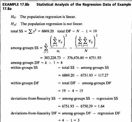
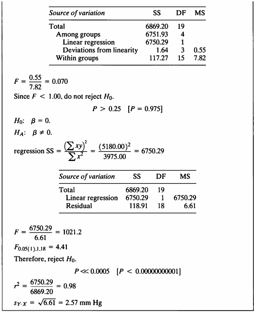
EXAMPLE 17.8a에서 구한 회귀모형의 선형성 검정을 위해 적합결여 F-test 를 수행하도록 하겠다.
선형성 검정을 하기 위해서는 단순 선형모형을 고려한 축소모형과 설명변수 각각의 값들을 factor화 하여 적합한 모형인 전체모형을 구한 뒤 Reduced model과 Full model 사이의 분산분석을 통하여 선형성을 검정한다.

Reduced model

rm <- lm(sbp~age,data=ex17_8)
summary(rm) %>% tidy %>% 
  rename("t value"="statistic","P value"="p.value") %>% 
  kable(caption = "Reduced model",booktabs = TRUE, valign = 't') %>%
  kable_styling(bootstrap_options = c("striped", "hover", "condensed", "responsive"))

Reduced model
term	estimate	std.error	t value	P value
(Intercept)	68.784906	2.2160746	31.03907	0
age	1.303145	0.0407667	31.96590	0

Full model

fm <- lm(sbp~factor(age),data=ex17_8)
summary(fm) %>% tidy %>% 
  rename("t value"="statistic","P value"="p.value") %>% 
  kable(caption = "Reduced model",booktabs = TRUE, valign = 't') %>%
  kable_styling(bootstrap_options = c("striped", "hover", "condensed", "responsive"))

Reduced model
term	estimate	std.error	t value	P value
(Intercept)	108.00000	1.614288	66.902558	0.00e+00
factor(age)40	12.50000	2.135502	5.853424	3.17e-05
factor(age)50	26.33333	2.282948	11.534793	0.00e+00
factor(age)60	39.20000	2.041931	19.197516	0.00e+00
factor(age)70	51.80000	2.041931	25.368146	0.00e+00

선형성 검정 (Lack-of-fit test)

\[\begin{aligned} H_0 &: The \ population \ regression \ is \ linear. \\ H_A &: The \ population \ regression \ is \ not \ linear. \end{aligned}\]

lof <- anova(rm,fm)
lof %>% tidy %>% 
  rename("Res df"="df.residual","RSS"="rss","Sum sq"="sumsq","F value"="statistic","P value"="p.value") %>% 
  kable(caption = "Reduced model",booktabs = TRUE, valign = 't') %>%
  kable_styling(bootstrap_options = c("striped", "hover", "condensed", "responsive"))

Reduced model
term	Res df	RSS	df	Sum sq	F value	P value
sbp \~ age	18	118.9107	NA	NA	NA	NA
sbp \~ factor(age)	15	117.2667	3	1.644025	0.0700977	0.9750327

적합결여 검정 결과 검정통계량 F값은 0.07, p-value=0.975 이므로 유의수준 0.05보다 커 귀무가설을 기각할 충분한 근거를 가지고있지 않다.
그러므로 유의수준 5%하에 모 회귀모델은 선형성을 따른다고 할 충분한 근거가 있다고 할 수 있다.

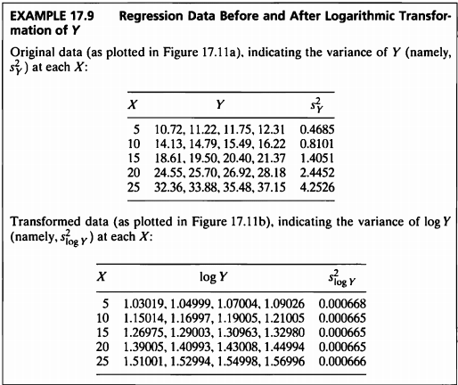
EXAMPLE 17.9

#데이터셋
X<-c(rep(5,4),rep(10,4),rep(15,4),rep(20,4),rep(25,4))
Y<-c(10.72,11.22,11.75,12.31,14.13,14.79,15.49,16.22,18.61,19.50,20.40,21.37, 24.55,25.70,26.92,28.18,32.36,33.88,35.48,37.15)

ex17_9 <- data.frame(X,Y)
ex17_9%>%
  kbl(caption = "Dataset of Example 17_9",escape=F) %>%
  kable_styling(bootstrap_options = c("striped", "hover", "condensed", "responsive"))

Dataset of Example 17_9
X	Y
5	10.72
5	11.22
5	11.75
5	12.31
10	14.13
10	14.79
10	15.49
10	16.22
15	18.61
15	19.50
15	20.40
15	21.37
20	24.55
20	25.70
20	26.92
20	28.18
25	32.36
25	33.88
25	35.48
25	37.15

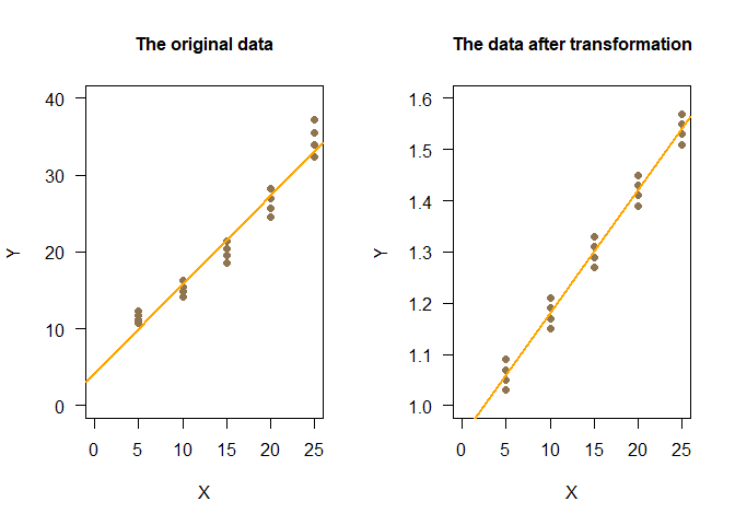
원 데이터와 로그변환한 데이터 간의 차이를 확인해보도록 하겠다.

로그변환

log_y <- log(Y,base=10)
ex17_9_trans <- data.frame(X,log_y)
ex17_9_trans%>%
  kbl(caption = "Logarithmic transformation Dataset of Example 17_9",escape=F) %>%
  kable_styling(bootstrap_options = c("striped", "hover", "condensed", "responsive"))

Logarithmic transformation Dataset of Example 17_9
X	log_y
5	1.030195
5	1.049993
5	1.070038
5	1.090258
10	1.150142
10	1.169968
10	1.190051
10	1.210051
15	1.269746
15	1.290035
15	1.309630
15	1.329805
20	1.390051
20	1.409933
20	1.430075
20	1.449941
25	1.510009
25	1.529943
25	1.549984
25	1.569959

ex17_9_result1 <- lm(Y~X, data=ex17_9)
#ex17.9_result1$residuals
ex17_9_result2 <- lm(log_y~X, data=ex17_9_trans)
#ex17.9_result2$residuals

par(mfrow=c(1,2))
plot(X, Y, pch=16,las=1,xlab="X", ylab="Y",ylim=c(0,40),xlim=c(0,25), main="The original data", cex.main=1, col="#8f7450")
abline(coef(ex17_9_result1), lwd=2, col="orange")
plot(X,log_y,pch=16,las=1,xlab="X",ylab="Y",ylim=c(1.0,1.6),xlim=c(0,25), main="The data after transformation", cex.main=1, col="#8f7450")
abline(coef(ex17_9_result2), lwd=2, col="orange")

par(mfrow=c(1,2))
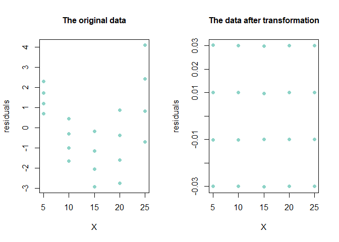
plot(X, ex17_9_result1$residuals, xlab="X", ylab="residuals", main = "The original data", cex.main=1, pch=16, col="#8dd3c7")
plot(X, ex17_9_result2$residuals, xlab="X", ylab="residuals", main = "The data after transformation", cex.main=1, pch=16, col="#8dd3c7")

par(mfrow=c(1,2))
qqnorm(ex17_9_result1$residuals, main = "The original data", cex.main=1, pch=16, col="#8dd3c7")
qqnorm(ex17_9_result2$residuals, main = "The data after transformation", cex.main=1, pch=16, col="#8dd3c7")

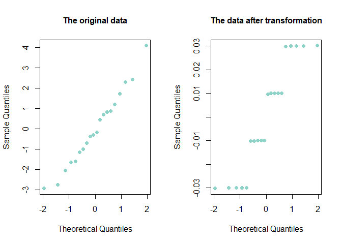
데이터를 로그변환하였을 때 더 강한 선형성을 가짐을 알 수 있다.
그리고 로그변환하였을 때의 잔차의 절대값이 변환 전보다 크게 줄었음을 알 수 있다.

origin <- c(var(Y[ex17_9$X==5]),var(Y[ex17_9$X==10]),var(Y[ex17_9$X==15]),var(Y[ex17_9$X==20]),var(Y[ex17_9$X==25])) 
logtrans <- c(var(log_y[ex17_9_trans$X==5]),var(log_y[ex17_9_trans$X==10]),var(log_y[ex17_9_trans$X==15]),var(log_y[ex17_9_trans$X==20]),var(log_y[ex17_9_trans$X==25])) 
variance <- data.frame(origin,logtrans)
variance%>%
  kbl(caption = "Variance of each of original data set Logarithmic transformation",escape=F) %>%
  kable_styling(bootstrap_options = c("striped", "hover", "condensed", "responsive"))

Variance of each of original data set Logarithmic transformation
origin	logtrans
0.4684667	0.0006682
0.8100917	0.0006654
1.4051333	0.0006652
2.4452250	0.0006654
4.2525583	0.0006659

SAS 프로그램 결과

SAS 접기/펼치기 버튼

17장

EXAMPLE 17.1

DATA ex17_1;
INPUT age wing @@;
CARDS;
3 1.4 4 1.5 5 2.2 6 2.4 8 3.1 9 3.2 
10 3.2 11 3.9 12 4.1 14 4.7 15 4.5 16 5.2 17 5
;
RUN;

PROC PRINT DATA=ex17_1;
RUN;

SAS 출력

SAS 시스템


OBS	age	wing
1	3	1.4
2	4	1.5
3	5	2.2
4	6	2.4
5	8	3.1
6	9	3.2
7	10	3.2
8	11	3.9
9	12	4.1
10	14	4.7
11	15	4.5
12	16	5.2
13	17	5.0

PROC SGPLOT DATA=ex17_1;
	REG y=wing x=age;
	INSET /	border title="Wing Lengths of 13 Sparrows of Various Ages." position=topleft;
RUN;

SAS 출력

EXAMPLE 17.2

ods graphics off;ods exclude all;ods noresults;
PROC REG DATA=ex17_1;
	MODEL wing=age;
	PLOT wing*age;
	ODS OUTPUT ParameterEstimates=ParameterEstimates;
RUN;
ods graphics on;ods exclude none;ods results;

PROC PRINT DATA=ParameterEstimates;
RUN;

SAS 출력

wing*age


OBS	Model	Dependent	Variable	DF	Estimate	StdErr	tValue	Probt
1	MODEL1	wing	Intercept	1	0.71309	0.14790	4.82	0.0005
2	MODEL1	wing	age	1	0.27023	0.01349	20.03	<.0001

EXAMPLE 17.3

ods graphics off;ods exclude all;ods noresults;
PROC REG DATA=ex17_1;
	MODEL wing=age;
	PLOT wing*age;
	ODS OUTPUT ANOVA=ANOVA FitStatistics=FitStatistics;
RUN;
ods graphics on;ods exclude none;ods results;

PROC PRINT DATA=ANOVA;
RUN;

PROC PRINT DATA= FitStatistics label;
RUN;

SAS 출력

wing*age


OBS	Model	Dependent	Source	DF	SS	MS	FValue	ProbF
1	MODEL1	wing	Model	1	19.13221	19.13221	401.09	<.0001
2	MODEL1	wing	Error	11	0.52471	0.04770	_	_
3	MODEL1	wing	Corrected Total	12	19.65692	_	_	_

wing*age


OBS	Model	Dependent	Label1	cValue1	nValue1	Label2	cValue2	nValue2
1	MODEL1	wing	Root MSE	0.21841	0.218405	R-Square	0.9733	0.973307
2	MODEL1	wing	Dependent Mean	3.41538	3.415385	Adj R-Sq	0.9709	0.970880
3	MODEL1	wing	Coeff Var	6.39475	6.394748			0

EXAMPLE 17.4

ods graphics off;ods exclude all;ods noresults;
PROC REG DATA=ex17_1;
   MODEL wing=age;
   ODS OUTPUT ParameterEstimates=PE;
RUN;

DATA pe1;
	SET pe;
	t=Estimate/StdErr;
RUN;
ods graphics on;ods exclude none;ods results;

PROC PRINT DATA=pe1;
	VAR Estimate StdErr t;
	WHERE Variable='age';
RUN;

SAS 출력

wing*age


OBS	Estimate	StdErr	t
2	0.27023	0.01349	20.0272

EXAMPLE 17.5

DATA ex17_5;
INPUT age @@;
CARDS;
13
;
RUN; 

DATA ex17_5f;
	SET ex17_5 ex17_1  ;
RUN;

ods graphics off; ods exclude all; ods noresults;
PROC REG DATA=ex17_5f; 
	MODEL wing=age / P CLM CLI ;
	ODS OUTPUT OutputStatistics=OutputStatistics;
RUN;
ods graphics on; ods exclude none; ods results;

PROC PRINT DATA=OutputStatistics LABEL;
	OPTIONS firstobs=1 obs=1;
	VAR StdErrMeanPredict LowerCLMean UpperCLMean;
RUN;

SAS 출력

wing*age


OBS	Std Err Mean Predict	Lower 95% CL Mean	Upper 95% CL Mean
1	0.0729	4.0657	4.3864

EXAMPLE 17.6

PROC IML;
	RESET nolog;
	y=4.225;
	s=0.073;
	t=(y-4)/s;
	p=1-probt(t,11);
	PRINT t p;
RUN;
QUIT;

SAS 출력

wing*age

t	p
3.0821918	0.0052152

EXAMPLE 17.7

PROC IML;
USE ex17_1;
READ all;
CLOSE ex17_1;

Yi = 4.5;
df = 11;
NObsUsed = nrow(wing);

x = repeat(1, nrow(age)) ||  age;
y = wing;
  n=nrow(x);                 
  k=ncol(x);                  
  xpx=x`*x;                   
  xpy=x`*y;
  xpxi=inv(xpx);            
  beta=xpxi*xpy;             
  sse = y`*y-xpy`*beta;   
  dfe = n-k;                  
  mse = sse/dfe;             
  rmse = sqrt(mse);          
  rsquare = 1-sse/((y-y[:])[##]);

  covb = mse#xpxi ;
  std_beta = SQRT(VECDIAG(covb)) ; 

  sy = std(y);
  Syx = sy * sqrt((1-rsquare)*(n-1)/(n-2));
  S2yx = Syx **2;
  xbar = mean(age);
  Sxx = (age- xbar)`*(age- xbar);
  
  Ybar=mean(y);

a = beta[1]; Sa=std_beta[1];
Byx = beta[2]; Sb=std_beta[2];
tvalue =  tinv(0.975, df);

prediced_X = (Yi-a) / Byx;
D = Byx**2 - (tvalue**2 * Sb**2);
H = (tvalue / D) * sqrt ( S2yx * (D * (1+(1/NObsUsed)) + ((Yi - Ybar)**2) / Sxx));

LL = Xbar + ((Byx * (Yi - Ybar)) / D) - H;
UL = Xbar + ((Byx * (Yi - Ybar)) / D) + H;

PRINT prediced_X LL UL;
RUN;
QUIT;

SAS 출력

wing*age

prediced_X	LL	UL
14.01369	12.152556	15.972963

EXAMPLE 17.8

DATA ex17_8;
INPUT x y @@;
CARDS;
30 108 30 110 30 106
40 125 40 120 40 118 40 119
50 132 50 137 50 134
60 148 60 151 60 146 60 147 60 144
70 162 70 156 70 164 70 158 70 159
;
RUN;

PROC REG DATA=ex17_8;;
	MODEL y=x / lackfit;
RUN;

SAS 출력

wing*age

The REG Procedure

Model: MODEL1

Dependent Variable: y


Number of Observations Read	20
Number of Observations Used	20


Analysis of Variance
Source	DF	Sum of Squares	Mean Square	F Value	Pr > F
Model	1	6750.28931	6750.28931	1021.82	<.0001
Error	18	118.91069	6.60615
Lack of Fit	3	1.64403	0.54801	0.07	0.9750
Pure Error	15	117.26667	7.81778
Corrected Total	19	6869.20000


Root MSE	2.57024	R-Square	0.9827
Dependent Mean	137.20000	Adj R-Sq	0.9817
Coeff Var	1.87336


Parameter Estimates
Variable	DF	Parameter Estimate	Standard Error	t Value	Pr > \|t\|
Intercept	1	68.78491	2.21607	31.04	<.0001
x	1	1.30314	0.04077	31.97	<.0001

wing*age

The REG Procedure

Model: MODEL1

Dependent Variable: y

Scatterplot of y by x overlaid with the fit line, a 95% confidence band and lower and upper 95% prediction limits.

EXAMPLE 17.9

DATA ex17_9 ; 
INPUT x y @@ ; 
CARDS; 
5 10.72 5 11.22 5 11.75 5 12.31
10 14.13 10 14.79 10 15.49 10 16.22
15 18.61 15 19.50 15 20.40 15 21.37
20 24.55 20 25.70 20 26.92 20 28.18
25 32.36 25 33.88 25 35.48 25 37.15
;
RUN;

DATA ex17_9_log;
    SET ex17_9;
    log_y = log10(y);
RUN;

PROC REG DATA=ex17_9_log;
    MODEL y=x;
    ODS SELECT ResidualPlot;
RUN;

PROC REG DATA=ex17_9_log;
    MODEL log_y=x;
    ODS SELECT ResidualPlot;
RUN;

SAS 출력

wing*age

The REG Procedure

Model: MODEL1

Dependent Variable: y

wing*age

The REG Procedure

Model: MODEL1

Dependent Variable: log_y

Scatter plot of residuals by x for log_y.

교재: Biostatistical Analysis (5th Edition) by Jerrold H. Zar

**이 글은 22학년도 1학기 의학통계방법론 과제 자료들을 정리한 글 입니다.**

age	sbp
30	108
30	110
30	106
40	125
40	120
40	118
40	119
50	132
50	137
50	134
60	148
60	151
60	146
60	147
60	144
70	162
70	156
70	164
70	158
70	159

OBS	age	wing
1	3	1.4
2	4	1.5
3	5	2.2
4	6	2.4
5	8	3.1
6	9	3.2
7	10	3.2
8	11	3.9
9	12	4.1
10	14	4.7
11	15	4.5
12	16	5.2
13	17	5.0

age	sbp
30	108
30	110
30	106
40	125
40	120
40	118
40	119
50	132
50	137
50	134
60	148
60	151
60	146
60	147
60	144
70	162
70	156
70	164
70	158
70	159

OBS	age	wing
1	3	1.4
2	4	1.5
3	5	2.2
4	6	2.4
5	8	3.1
6	9	3.2
7	10	3.2
8	11	3.9
9	12	4.1
10	14	4.7
11	15	4.5
12	16	5.2
13	17	5.0

Simple Linear Regression

R 프로그램 결과

17장

EXAMPLE 17.1

EXAMPLE 17.2

EXAMPLE 17.3

EXAMPLE 17.4

EXAMPLE 17.5

EXAMPLE 17.6

EXAMPLE 17.7

EXAMPLE 17.8a

EXAMPLE 17.8b

EXAMPLE 17.9

SAS 프로그램 결과

17장

EXAMPLE 17.1

EXAMPLE 17.2

EXAMPLE 17.3

EXAMPLE 17.4

EXAMPLE 17.5

EXAMPLE 17.6

EXAMPLE 17.7

EXAMPLE 17.8

EXAMPLE 17.9

Templates (for web app):

Error

age	sbp
30	108
30	110
30	106
40	125
40	120
40	118
40	119
50	132
50	137
50	134
60	148
60	151
60	146
60	147
60	144
70	162
70	156
70	164
70	158
70	159

OBS	age	wing
1	3	1.4
2	4	1.5
3	5	2.2
4	6	2.4
5	8	3.1
6	9	3.2
7	10	3.2
8	11	3.9
9	12	4.1
10	14	4.7
11	15	4.5
12	16	5.2
13	17	5.0