[의학통계방법론] Ch12. Two-Factor Analysis of Variance

28 Apr 2022 in Study log / Study / 의학통계방법론 on R, Sas, Blog, Jekyll, Jupyter, Data, Python

Two-Factor Analysis of Variance
R 프로그램 결과
- 12장
SAS 프로그램 결과
- 12장

Two-Factor Analysis of Variance

예제 데이터파일 다운로드

R 프로그램 결과

R 접기/펼치기 버튼

패키지

설치된 패키지 접기/펼치기 버튼

getwd()

## [1] "C:/Biostat"

library("readxl")
library("dplyr")
library("kableExtra")
library("broom")
library("ggplot2")
library("agricolae")
library("nonpar")

엑셀파일불러오기

#모든 시트를 하나의 리스트로 불러오는 함수
read_excel_allsheets <- function(file, tibble = FALSE) {
  sheets <- readxl::excel_sheets(file)
  x <- lapply(sheets, function(X) readxl::read_excel(file, sheet = X))
  if(!tibble) x <- lapply(x, as.data.frame)
  names(x) <- sheets
  x
}

12장

12장 연습문제 불러오기

#data_chap12에 연습문제 12장 모든 문제 저장
data_chap12 <- read_excel_allsheets("data_chap12.xls")

#연습문제 각각 데이터 생성
for (x in 1:length(data_chap12)){
  assign(paste0('ex12_',c(1,4,5,6))[x],data_chap12[x])
  }

#연습문제 데이터 형식을 리스트에서 데이터프레임으로 변환
for (x in 1:length(data_chap12)){
  assign(paste0('ex12_',c(1,4,5,6))[x],data.frame(data_chap12[x]))
  }

EXAMPLE 12.1

#데이터셋
ex12_1%>%
  kbl(caption = "Dataset",escape=F) %>%
  kable_styling(bootstrap_options = c("striped", "hover", "condensed", "responsive"))

Dataset
exam12_1.No	exam12_1.Hormone	exam12_1.Sex	exam12_1.plasma_calcium
1	No Hormone	Female	16.3
2	No Hormone	Female	20.4
3	No Hormone	Female	12.4
4	No Hormone	Female	15.8
5	No Hormone	Female	9.5
6	No Hormone	Male	15.3
7	No Hormone	Male	17.4
8	No Hormone	Male	10.9
9	No Hormone	Male	10.3
10	No Hormone	Male	6.7
11	Yes Hormone	Female	38.1
12	Yes Hormone	Female	26.2
13	Yes Hormone	Female	32.3
14	Yes Hormone	Female	35.8
15	Yes Hormone	Female	30.2
16	Yes Hormone	Male	34.0
17	Yes Hormone	Male	22.8
18	Yes Hormone	Male	27.8
19	Yes Hormone	Male	25.0
20	Yes Hormone	Male	29.3

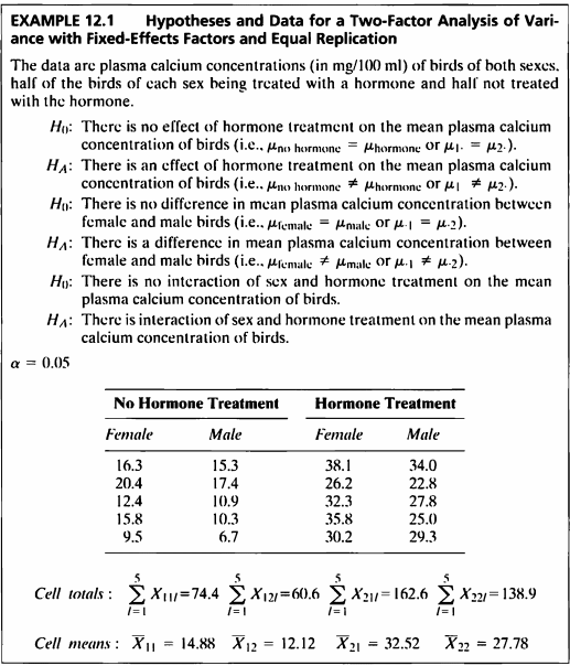
해당 데이터는 성별에 따른 새의 혈청 내 칼슘 농도를 기록한 데이터이다.
호르몬 치료 유무와 성별에 따른 혈청 내 칼슘 농도에 차이가 있는지 이요인 분산분석을 시행한다.

\[\begin{aligned} H_0 &: There\ is\ no\ effect\ of\ hormone\ treatment\ on\ the\ mean\ plasma\ calcium\ concentration\ of\ birds\ \\ H_A &: There\ is\ an\ effect\ of\ hormone\ treatment\ on\ the\ mean\ plasma\ calcium\ concentration\ of\ birds\ \\ \\ H_0 &: There\ is\ no\ difference\ \ in\ mean\ plasma\ calcium\ concentration\ between\ female\ and\ male\ birds\ \\ H_A &: There\ is\ a\ difference\ \ in\ mean\ plasma\ calcium\ concentration\ between\ female\ and\ male\ birds\ \\ \\ H_0 &: There\ is\ no\ interaction\ of\ sex\ and\ hormone\ treatment\ on\ the\ mean\ plasma\ calcium\ concentration\ of\ birds\ \\ H_A &: There\ is\ interaction\ of\ sex\ and\ hormone\ treatment\ on\ the\ mean\ plasma\ calcium\ concentration\ of\ birds\ \\ \end{aligned}\]

nf <- subset(ex12_1$exam12_1.plasma_calcium, ex12_1$exam12_1.Hormone=="No Hormone" & ex12_1$exam12_1.Sex=="Female")
nm <- subset(ex12_1$exam12_1.plasma_calcium, ex12_1$exam12_1.Hormone=="No Hormone" & ex12_1$exam12_1.Sex=="Male")
yf <- subset(ex12_1$exam12_1.plasma_calcium, ex12_1$exam12_1.Hormone=="Yes Hormone" & ex12_1$exam12_1.Sex=="Female")
ym <- subset(ex12_1$exam12_1.plasma_calcium, ex12_1$exam12_1.Hormone=="Yes Hormone" & ex12_1$exam12_1.Sex=="Male")
ex12_1a <- data.frame(no_hormone_female=nf,no_hormone_male=nm,yes_hormone_female=yf,yes_hormone_male=ym)
ex12_1a%>%
  kbl(caption = "Dataset of ex12_1") %>%
  kable_styling(bootstrap_options = c("striped", "hover", "condensed", "responsive"))

Dataset of ex12_1
no_hormone_female	no_hormone_male	yes_hormone_female	yes_hormone_male
16.3	15.3	38.1	34.0
20.4	17.4	26.2	22.8
12.4	10.9	32.3	27.8
15.8	10.3	35.8	25.0
9.5	6.7	30.2	29.3

cell_totals <- c(sum(nf),sum(nm),sum(yf),sum(ym))
cell_means <- c(mean(nf),mean(nm),mean(yf),mean(ym))
cell <- data.frame(rbind(cell_totals,cell_means))
names(cell) <- c("X_11","X_12","X_21","X_22")
cell%>%
  kbl(caption = "Cell totals and Cell means") %>%
  kable_styling(bootstrap_options = c("striped", "hover", "condensed", "responsive"))

Cell totals and Cell means
	X_11	X_12	X_21	X_22
cell_totals	74.40	60.60	162.60	138.90
cell_means	14.88	12.12	32.52	27.78

EXAMPLE 12.1a

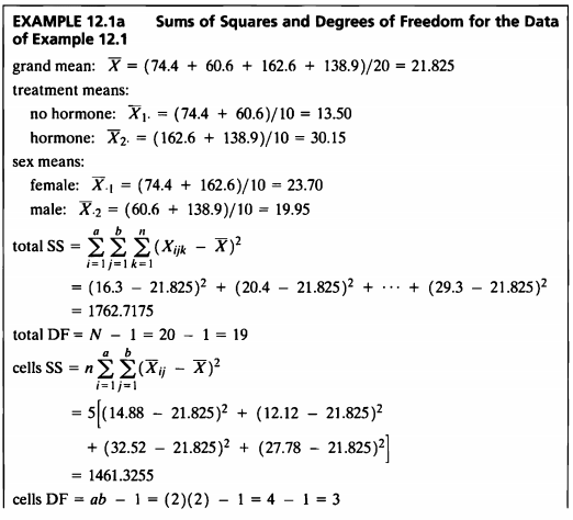
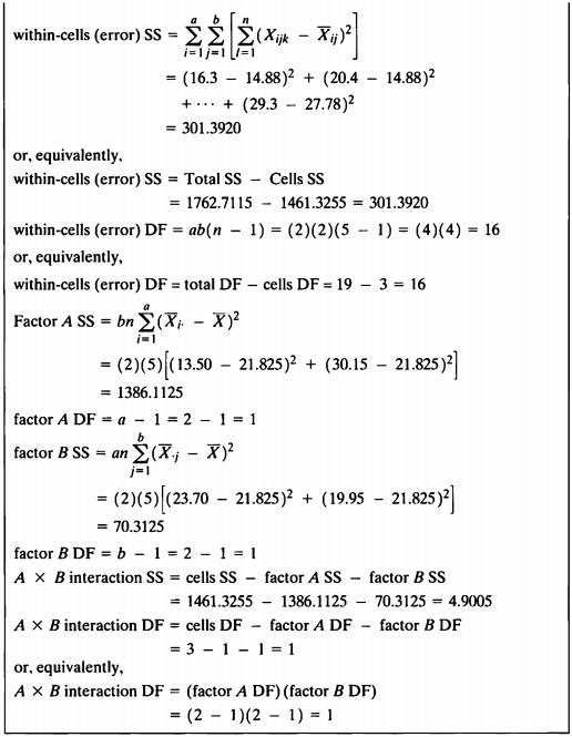
예제에서 나온 식으로 제곱합 및 자유도를 구하는 함수를 직접 작성하여 ANOVA table을 작성하여 보았다.

f12_1a <- function(x){
  N <- (length(x)*nrow(x))
  grand_mean <- sum(x)/N
  no_hormone_means <- sum(x[,1:2])/10
  hormone_means <- sum(x[,3:4])/10
  female_means <- sum(x[,c(1,3)])/10
  male_means <- sum(x[,c(2,4)])/10
  total_SS <- sum((x-grand_mean)^2)
  total_DF <- N-1
  cells <- vector()
  for (i in 1:4){
    cells[i] <- (mean(ex12_1a[,i]) - grand_mean)^2
  }
  cells_SS <- sum(5*cells)
  cells_DF <- 3
  within_cells_SS <- total_SS - cells_SS
  within_cells_DF <- total_DF - cells_DF
  Factor_A_SS <- 2*5*((no_hormone_means-grand_mean)^2+(hormone_means-grand_mean)^2)
  Factor_A_DF <- 1
  Factor_B_SS <- 2*5*((female_means-grand_mean)^2+(male_means-grand_mean)^2)
  Factor_B_DF <- 1
  AXB_interaction_SS <- cells_SS-Factor_A_SS-Factor_B_SS
  AXB_interaction_DF <- cells_DF - Factor_A_DF - Factor_B_DF
  SS <- c(total_SS,cells_SS,Factor_A_SS,Factor_B_SS,round(AXB_interaction_SS,4),round(within_cells_SS,4))
  DF <- c(total_DF,cells_DF,Factor_A_DF,Factor_B_DF,AXB_interaction_DF,within_cells_DF)
  source <- c("Total","Cells","Factor A (hormone)","Facor B (sex)","A X B","Within-Cells (Error)")
  MS <- c("","",Factor_A_SS/Factor_A_DF,Factor_B_SS/Factor_B_DF,round(AXB_interaction_SS/AXB_interaction_DF,4),within_cells_SS/within_cells_DF)
  res <- data.frame(source,SS,DF,MS)
  return(res)
}

f12_1a(ex12_1a)%>%
  kbl(caption = "Analysis of Variance Summary table") %>%
  kable_styling(bootstrap_options = c("striped", "hover", "condensed", "responsive"))

Analysis of Variance Summary table
source	SS	DF	MS
Total	1762.7175	19
Cells	1461.3255	3
Factor A (hormone)	1386.1125	1	1386.1125
Facor B (sex)	70.3125	1	70.3125
A X B	4.9005	1	4.9005
Within-Cells (Error)	301.3920	16	18.837

EXAMPLE 12.2

ex12_1$Hormone <- as.factor(ex12_1$exam12_1.Hormone)
ex12_1$Sex <- as.factor(ex12_1$exam12_1.Sex)

이원분산분석을 진행하기 전에 정규성과 등분산성, 독립성을 만족하는지 부터 확인하도록 한다.

Shapiro-Wilk Test로 그룹별 정규성을 평가하였다.

ex12_1 %>% group_by(exam12_1.Hormone, exam12_1.Sex) %>%
  summarise(shapiro_test = shapiro.test(exam12_1.plasma_calcium)$p.value)

## # A tibble: 4 × 3
## # Groups:   exam12_1.Hormone [2]
##   exam12_1.Hormone exam12_1.Sex shapiro_test
##   <chr>            <chr>               <dbl>
## 1 No Hormone       Female              0.931
## 2 No Hormone       Male                0.800
## 3 Yes Hormone      Female              0.949
## 4 Yes Hormone      Male                0.926

4그룹 모두 p-value가 0.05보다 매우 크므로 모집단이 정규성을 따르지 않는다는 대립가설을 채택할 충분한 근거가 없다.
따라서 정규성을 만족한다는 사실을 바탕으로 등분산성 검정을 진행한다.

Bartlett’s Test를 통해 등분산성 검정을 진행하였다.

bartlett.test(ex12_1$exam12_1.plasma_calcium~ex12_1$exam12_1.Hormone)

## 
##  Bartlett test of homogeneity of variances
## 
## data:  ex12_1$exam12_1.plasma_calcium by ex12_1$exam12_1.Hormone
## Bartlett's K-squared = 0.19987, df = 1, p-value = 0.6548

bartlett.test(ex12_1$exam12_1.plasma_calcium~ex12_1$exam12_1.Sex)

## 
##  Bartlett test of homogeneity of variances
## 
## data:  ex12_1$exam12_1.plasma_calcium by ex12_1$exam12_1.Sex
## Bartlett's K-squared = 0.091482, df = 1, p-value = 0.7623

p-value가 모두 0.05보다 크므로 등분산성이 아니라는 대립가설을 채택할 근거가 없다.

첫번째 가설

f12_2_1 <- function(x){
  f <- f12_1a(x)$SS[3]/as.numeric(f12_1a(x)$MS[6])
  f_0.05 <- qf(0.95,1,16)
  p_value <- 1-pf(f,1,16)
  if (f<f_0.05){
    reject_H0 <- "No"
  }else{
    reject_H0 <- "Yes"
  }
  res <- data.frame(f,f_0.05,p_value,reject_H0)
  return(res)
}

f12_2_1(ex12_1a)%>%
  kbl(caption = "Result of hypotheses for Hormone treatment") %>%
  kable_styling(bootstrap_options = c("striped", "hover", "condensed", "responsive"))

Result of hypotheses for Hormone treatment
f	f_0.05	p_value	reject_H0
73.58457	4.493999	2e-07	Yes

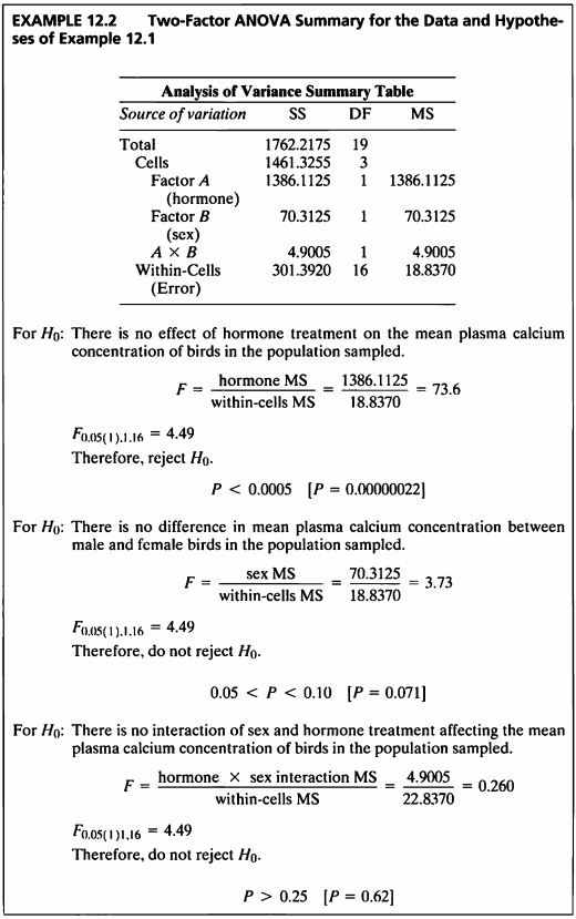
F-값이 73.6으로 임계값 4.49보다 큰 값이 나왔고, p-value가 0.05보다 매우 작으므로 유의수준 5%하에 귀무가설을 기각한다.
따라서 호르몬 치료에 따른 혈청 내 칼슘 함량의 평균이 다르다고 할 수 있다.

두번째 가설

\[\begin{aligned} H_0 &: There\ is\ no\ difference\ \ in\ mean\ plasma\ calcium\ concentration\ between\ female\ and\ male\ birds\ \\ H_A &: There\ is\ a\ difference\ \ in\ mean\ plasma\ calcium\ concentration\ between\ female\ and\ male\ birds\ \\ \end{aligned}\]

f12_2_2 <- function(x){
  f <- f12_1a(x)$SS[4]/as.numeric(f12_1a(x)$MS[6])
  f_0.05 <- qf(0.95,1,16)
  p_value <- 1-pf(f,1,16)
  if (f<f_0.05){
    reject_H0 <- "No"
  }else{
    reject_H0 <- "Yes"
  }
  res <- data.frame(f,f_0.05,p_value,reject_H0)
  return(res)
}

f12_2_2(ex12_1a)%>%
  kbl(caption = "Result of hypotheses for sex") %>%
  kable_styling(bootstrap_options = c("striped", "hover", "condensed", "responsive"))

Result of hypotheses for sex
f	f_0.05	p_value	reject_H0
3.73268	4.493999	0.0712638	No

F-값이 3.73으로 임계값 4.49보다 작은 값이 나왔고, p-value가 0.05보다 크므로 유의수준 5%하에 귀무가설을 기각할 수 없다.
따라서 성별에 따른 혈청 내 칼슘 함량의 평균이 다르다고 할 수 없다.

세번째 가설

\[\begin{aligned} H_0 &: There\ is\ no\ interaction\ of\ sex\ and\ hormone\ treatment\ on\ the\ mean\ plasma\ calcium\ concentration\ of\ birds\ \\ H_A &: There\ is\ interaction\ of\ sex\ and\ hormone\ treatment\ on\ the\ mean\ plasma\ calcium\ concentration\ of\ birds\ \\ \end{aligned}\]

f12_2_3 <- function(x){
  f <- f12_1a(x)$SS[5]/as.numeric(f12_1a(x)$MS[6])
  f_0.05 <- qf(0.95,1,16)
  p_value <- 1-pf(f,1,16)
  if (f<f_0.05){
    reject_H0 <- "No"
  }else{
    reject_H0 <- "Yes"
  }
  res <- data.frame(f,f_0.05,p_value,reject_H0)
  return(res)
}

f12_2_3(ex12_1a)%>%
  kbl(caption = "Result of hypotheses for interaction") %>%
  kable_styling(bootstrap_options = c("striped", "hover", "condensed", "responsive"))

Result of hypotheses for interaction
f	f_0.05	p_value	reject_H0
0.2601529	4.493999	0.6169788	No

F-값이 0.26으로 임계값 4.49보다 작은 값이 나왔고, p-value가 0.05보다 크므로 유의수준 5%하에 귀무가설을 기각할 수 없다.
따라서 호르몬과 성별의 교호작용 효과가 있다고 할 수 없다.

aov()를 사용하여 이원분산분석을 실시한다.

library(broom)
aov(exam12_1.plasma_calcium~exam12_1.Hormone*exam12_1.Sex, data=ex12_1) %>% 
  tidy() %>% 
  rename(" "="term","Sum Sq"="sumsq","Mean Sq"="meansq","F value"="statistic","Pr(>F)"="p.value") %>% 
  kable(caption = "Two-factor ANOVA",booktabs = TRUE, valign = 't')%>%
  kable_styling(bootstrap_options = c("striped", "hover", "condensed", "responsive"))

Two-factor ANOVA
	df	Sum Sq	Mean Sq	F value	Pr(\>F)
exam12_1.Hormone	1	1386.1125	1386.1125	73.5845676	0.0000002
exam12_1.Sex	1	70.3125	70.3125	3.7326804	0.0712638
exam12_1.Hormone:exam12_1.Sex	1	4.9005	4.9005	0.2601529	0.6169788
Residuals	16	301.3920	18.8370	NA	NA

stripchart() 함수로 1차원 산점도를 확인하여 본다.

par(mfrow=c(1,2))
stripchart(ex12_1$exam12_1.plasma_calcium~ex12_1$exam12_1.Hormone , vertical=T, xlab="Hormone", ylab="calcium", method="jitter", col="#8dd3c7", pch=16) 
stripchart(ex12_1$exam12_1.plasma_calcium~ex12_1$exam12_1.Sex, vertical=T, xlab="Female / male", ylab="calcium", method="jitter", col="#007266", pch=16)

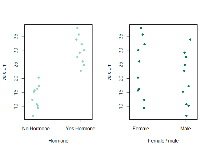
stripchart() 함수는 sample size가 작을 때 box plot을 대신하기 좋다.

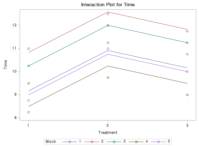
interaction.plot(ex12_1$exam12_1.Hormone,ex12_1$exam12_1.Sex,ex12_1$exam12_1.plasma_calcium, col=c("orange","#8f7450"), bty="l",  main="interaction  plot",  xlab="Hormone",  ylab="mean  of calcium", trace.label = "Sex")

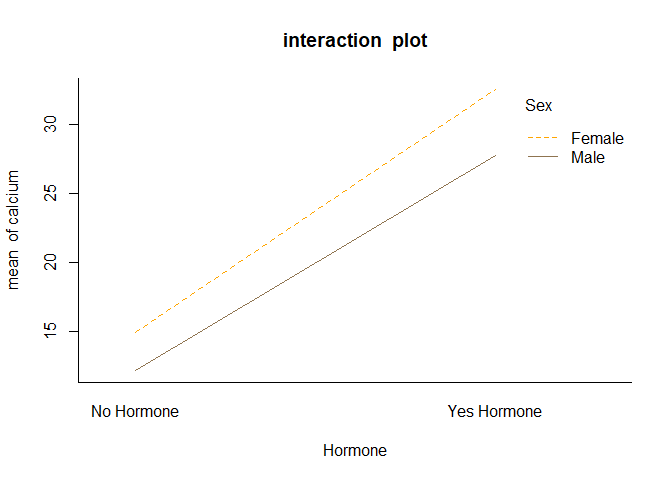
교호작용 그래프를 보면 서로 겹치는 부분이 없어 성별과 호르몬 간 교호작용이 존재하지 않음을 확인할 수 있으며, 성별이 여자이고 호르몬치료를 받았을 때 혈청 내 칼슘의 농도가 최대가 됨을 알 수 있다.

EXAMPLE 12.2a

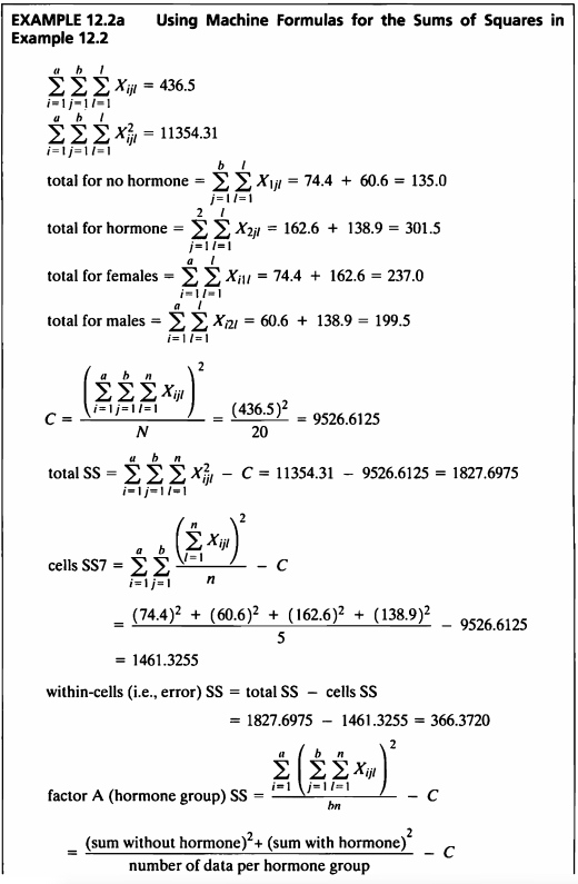
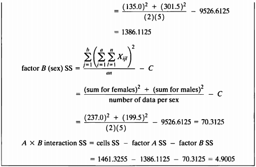
“Machine Formulas”라는 사용하여 Example 12.1a에서 구한 결과와 같은 값을 구하여 보자.

f12_2a <- function(x){
  N <- (length(x)*nrow(x))
  Xi <- sum(x) 
  Xi2 <- sum(x^2)
  C <- sum(x)^2/N
  no_hormone <- sum(x[,1:2])
  hormone <- sum(x[,3:4])
  females <- sum(x[,c(1,3)])
  males <- sum(x[,c(2,4)])
  total_SS <- Xi2-C
  aa <- vector()
  for (i in 1:4){
    aa[i] <- sum(ex12_1a[i])^2
  }
  cells_SS7 <- (sum(aa)/5) -C
  within_cells_SS <- total_SS-cells_SS7
  Factor_A_SS <- ((no_hormone^2+hormone^2)/10)-C
  Factor_B_SS <- ((females^2+males^2)/10)-C
  AXB_interaction_SS <- cells_SS7-Factor_A_SS-Factor_B_SS
  res <- data.frame(total_SS,cells_SS7,within_cells_SS,Factor_A_SS,Factor_B_SS,AXB_interaction_SS)
  return(res)
}

f12_2a(ex12_1a)%>%
  kbl(caption = "Result of Machine formula") %>%
  kable_styling(bootstrap_options = c("striped", "hover", "condensed", "responsive"))

Result of Machine formula
total_SS	cells_SS7	within_cells_SS	Factor_A\_SS	Factor_B\_SS	AXB_interaction_SS
1762.717	1461.325	301.392	1386.112	70.3125	4.9005

EXAMPLE 12.3

Xbar_1 = mean(ex12_1[ex12_1$exam12_1.Hormone=="No Hormone",]$exam12_1.plasma_calcium)
Xbar_2 = mean(ex12_1[ex12_1$exam12_1.Hormone=="Yes Hormone",]$exam12_1.plasma_calcium)
No.Hormone = ex12_1[ex12_1$exam12_1.Hormone=="No Hormone",]$exam12_1.plasma_calcium
Yes.Hormone = ex12_1[ex12_1$exam12_1.Hormone=="Yes Hormone",]$exam12_1.plasma_calcium
Female=ex12_1[ex12_1$exam12_1.Sex=="Female",]$exam12_1.plasma_calcium
Male=ex12_1[ex12_1$exam12_1.Sex=="Male",]$exam12_1.plasma_calcium
Xbar_pooled = (sum(Female)+sum(Male))/(length(Female)+length(Male))

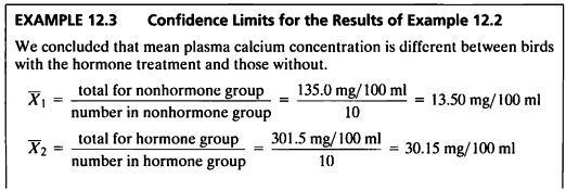
호르몬을 처리하지 않은 새들의 plasma calcium 농도의 표본평균은 13.50mg/100ml이고,
호르몬을 처리한 새들의 plasma calcium 농도의 표본평균은 30.15 mg/100ml이었다.

CI_ex12 <- function(x){
  exam12_3_results = vector()
  sample.mean <- mean(x)
  exam12_3_results <- c(exam12_3_results, "mean"=sample.mean)
  sample.s2 <- 18.8370
  sample.n <- length(x)
  t.score = round(qt(p=0.05/2, df=16,lower.tail=F),3)
  margin.error <- t.score * sqrt(sample.s2/sample.n)
  lower.bound <- round(sample.mean - margin.error, 2)
  upper.bound <- round(sample.mean + margin.error, 2)
  CI = paste(lower.bound, ",", upper.bound)
  exam12_3_results <- c(exam12_3_results, "95% CI"=CI)
  exam12_3_results <- as.data.frame(exam12_3_results)
  return(exam12_3_results)
}

CI_ex12(No.Hormone)

##        exam12_3_results
## mean               13.5
## 95% CI    10.59 , 16.41

CI_ex12(Yes.Hormone)

##        exam12_3_results
## mean              30.15
## 95% CI    27.24 , 33.06

CI_ex12(Female)

##        exam12_3_results
## mean               23.7
## 95% CI    20.79 , 26.61

CI_ex12(Male)

##        exam12_3_results
## mean              19.95
## 95% CI    17.04 , 22.86

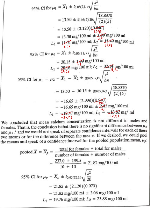
호르몬을 처리하지 않은 새들의 plasma calcium 농도의 모평균에 대한 95% 신뢰구간 (10.59mg/100ml , 16.41mg/100ml)
호르몬 처리를 한 새들의 plasma calcium 농도의 모평균에 대한 95% 신뢰구간 (27.24mg/100ml, 33.06mg/100ml)
암컷 새들의 plasma calcium 농도의 모평균에 대한 95% 신뢰구간 (20.79mg/100ml, 26.61mg/100ml)
수컷 새들의 plasma calcium 농도의 모평균에 대한 95% 신뢰구간 (17.04mg/100ml, 22.86mg/100ml)

CI_ex12_difference <- function(x){
  exam12_3_results = vector()
  sample.mean <- mean(x)
  exam12_3_results <- c(exam12_3_results, "mean"=sample.mean)
  sample.s2 <- 18.8370
  sample.n <- length(x)
  q.score = round(qtukey(p=0.95,2,16),3)
  margin.error <- q.score * sqrt(sample.s2/sample.n)
  lower.bound <- round(sample.mean - margin.error, 2)
  upper.bound <- round(sample.mean + margin.error, 2)
  CI = paste(lower.bound, ",", upper.bound)
  exam12_3_results <- c(exam12_3_results, "95% CI"=CI)
  exam12_3_results <- as.data.frame(exam12_3_results)
  return(exam12_3_results)
}

CI_ex12_difference(No.Hormone - Yes.Hormone)

##        exam12_3_results
## mean             -16.65
## 95% CI  -20.76 , -12.54

CI_ex12_difference(Female - Male)

##        exam12_3_results
## mean               3.75
## 95% CI     -0.36 , 7.86

호르몬을 처리하지 않은 새들의 plasma calcium 농도의 모평균과 호르몬 처리를 한 새들의 plasma calcium 농도의 모평균의 차에 대한 95% 신뢰구간 (-20.76mg/100ml, -12.54mg/100ml)
신뢰구간이 0을 포함하지 않으므로 유의수준 5%하에 호르몬 처리에 따라 새들의 plasma calcium 농도의 모평균에는 차이가 있다고 볼 수 있다.
암컷 새들의 plasma calcium 농도의 모평균과 수컷 새들의 plasma calcium 농도의 모평균의 차에 대한 95% 신뢰구간 (-0.36mg/100ml, 7.86mg/100ml)
신뢰구간이 0을 포함하므로, 유의수준 5%하에 plasma calcium 농도의 모평균은 암컷과 수컷 새들 간에 유의미한 차이가 없다고 말할 수 있다.

CI_ex12_pooled <- function(x){
  exam12_3_pooled = vector()
  exam12_3_pooled = c(exam12_3_pooled, "Xbar_pooed"=x)
  t.score = qt(p=0.05/2, df=16,lower.tail=F)
  s2=18.8370
  margin = t.score * sqrt(s2/(length(Female)+length(Male)))
  lower.bound = round(x - margin, 3) 
  upper.bound = round(x + margin, 3) 
  CI = paste(lower.bound, ",", upper.bound)
  exam12_3_results <- c(exam12_3_pooled, "95% CI"=CI)
  exam12_3_results <- as.data.frame(exam12_3_results)
  return(exam12_3_results)
}

CI_ex12_pooled(Xbar_pooled)

##            exam12_3_results
## Xbar_pooed           21.825
## 95% CI      19.768 , 23.882

pooled population mean에 대한 95% 신뢰구간은 (19.76mg/100ml, 23.88mg/100ml)이다.

EXAMPLE 12.4

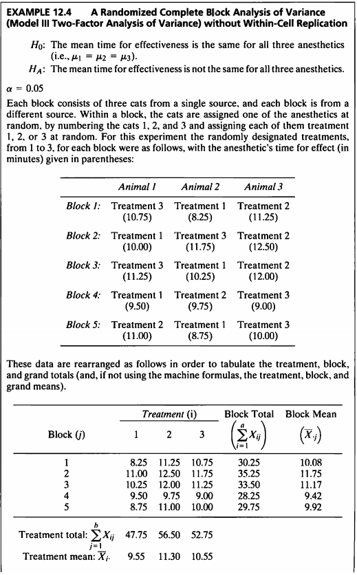
해당 데이터는 5개의 블록으로 구성되어 있으며, 한 블록에 세 마리의 고양이로 구성되어있다.
한 블록 안에서 고양이들은 세가지 마취제 중 하나를 무작위로 배정받는다.
배정받은 마취제의 효과 시간(분)을 기록한 데이터이다.
블록 내에 마취제를 투여함에 있어서는 반복을 하지 않으며, 고양이들이 랜덤으로 설정되었으며 이러한 반복이 없는 경우를 난괴법(Randomized Block Design)이라 한다.

#데이터셋
ex12_4%>%
  kbl(caption = "Dataset",escape=F) %>%
  kable_styling(bootstrap_options = c("striped", "hover", "condensed", "responsive"))

Dataset
exam12_4.Treatment	exam12_4.Block	exam12_4.Time
1	1	8.25
1	2	11.00
1	3	10.25
1	4	9.50
1	5	8.75
2	1	11.25
2	2	12.50
2	3	12.00
2	4	9.75
2	5	11.00
3	1	10.75
3	2	11.75
3	3	11.25
3	4	9.00
3	5	10.00

library(ggplot2)
ex12_4$exam12_4.Treatment <- as.factor(ex12_4$exam12_4.Treatment)
ex12_4$exam12_4.Block <- as.factor(ex12_4$exam12_4.Block)

ggplot(ex12_4, aes(x = exam12_4.Block, y = exam12_4.Time, fill=exam12_4.Block)) +
  geom_boxplot()+
  ggtitle("Boxplot of Time by Block")

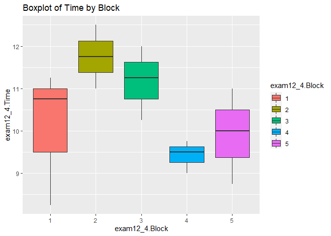
블록의 따른 마취 지속효과를 박스플롯으로 확인하여 보았다.

ggplot(ex12_4, aes(x = exam12_4.Treatment, y = exam12_4.Time, fill=exam12_4.Treatment)) +
  geom_boxplot()+
  ggtitle("Boxplot of Time by Treatment")

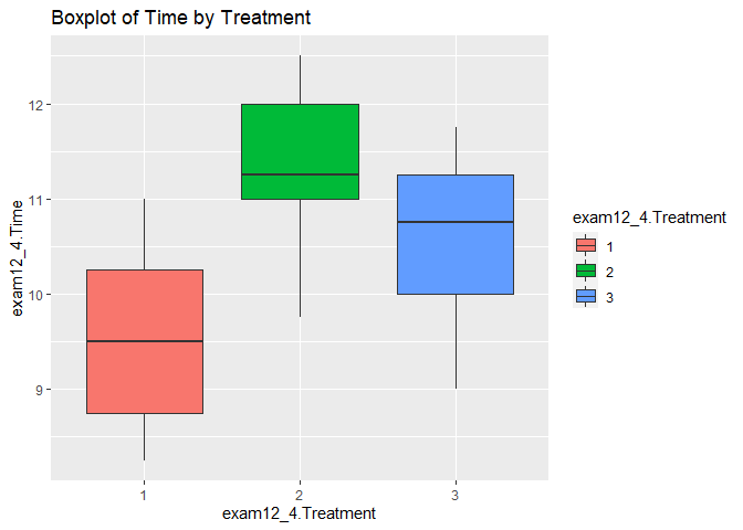
마취제의 따른 마취 지속효과를 박스플롯으로 확인하여 보았다.

Shapiro-Wilk Test로 정규성을 평가하였다.

shapiro.test(ex12_4$exam12_4.Time)

## 
##  Shapiro-Wilk normality test
## 
## data:  ex12_4$exam12_4.Time
## W = 0.97427, p-value = 0.9155

p-value가 0.05보다 매우 크므로 모집단이 정규성을 따르지 않는다는 대립가설을 채택할 충분한 근거가 없다.
따라서 정규성을 만족한다는 사실을 바탕으로 등분산성 검정을 진행한다.

Bartlett’s Test를 통해 등분산성 검정을 진행하였다.

bartlett.test(ex12_4$exam12_4.Time~ex12_4$exam12_4.Treatment)

## 
##  Bartlett test of homogeneity of variances
## 
## data:  ex12_4$exam12_4.Time by ex12_4$exam12_4.Treatment
## Bartlett's K-squared = 0.01031, df = 2, p-value = 0.9949

p-value가 모두 0.05보다 크므로 등분산성이 아니라는 아니라는 대립가설을 채택할 근거가 없다.
본 검정의 가설은 다음과 같다.

\[\begin{aligned} H_0 &:The\ mean\ time\ for\ effectiveness\ is\ the\ same\ for\ all\ three\ anesthetics. \\ H_A &: The\ mean\ time\ for\ effectiveness\ is\ not\ the\ same\ for\ all\ three\ anesthetics. \end{aligned}\]

Randomized Complete Block ANOVA

aov(exam12_4.Time~exam12_4.Treatment+exam12_4.Block, data = ex12_4) %>% 
  tidy() %>% 
  rename(" "="term","Sum Sq"="sumsq","Mean Sq"="meansq","F value"="statistic","Pr(>F)"="p.value") %>% 
  kable(caption = "Randomized Complete Block ANOVA",booktabs = TRUE, valign = 't') %>% 
  kable_styling(bootstrap_options = c("striped", "hover", "condensed", "responsive"))

Randomized Complete Block ANOVA
	df	Sum Sq	Mean Sq	F value	Pr(\>F)
exam12_4.Treatment	2	7.708333	3.8541667	10.42254	0.0059166
exam12_4.Block	4	11.066667	2.7666667	7.48169	0.0082277
Residuals	8	2.958333	0.3697917	NA	NA

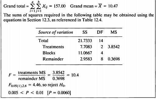
블록이 있는 분산분석을 수행한 결과이다.
분산분석 결과를 보면 Treatement와 블록의 p-value는 모두 0.05 보다 작으므로 귀무가설을 기각할 충분한 근거를 가지고 있다.
그러므로 마취약에 따라 마취의 효과 시간에 대한 모평균이 다르다라고 할 수 있다.

EXAMPLE 12.5

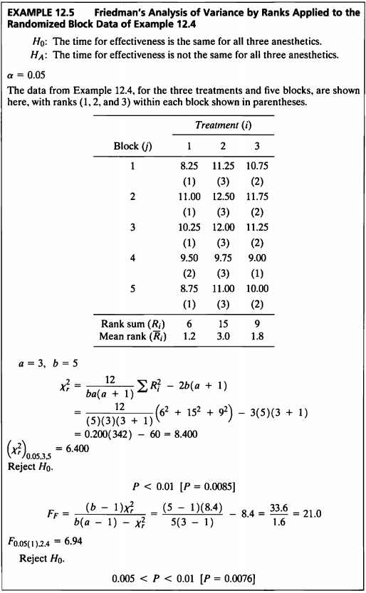
Example 12.4의 데이터를 사용하여 비모수적 방법인 Friedman’s test를 수행하도록 한다.
이 검정 방법은 각 블록 내에 있는 Treatment 즉, 마취제의 효과가 있는 시간에 대한 평균을 가지고 Rank를 매긴다.

Friedman’s Test

library(agricolae)
fr <- friedman(ex12_4$exam12_4.Block, trt=ex12_4$exam12_4.Treatment, ex12_4$exam12_4.Time, alpha=0.05)
  kable(fr[[1]], caption = paste0("Friedman's Test"))%>%
  kable_styling(bootstrap_options = c("striped", "hover", "condensed", "responsive"));kable(fr[[2]], caption = paste0("Parameters"))%>%
  kable_styling(bootstrap_options = c("striped", "hover", "condensed", "responsive"));kable(fr[[3]], caption = paste0("Means"))%>%
  kable_styling(bootstrap_options = c("striped", "hover", "condensed", "responsive"));kable(fr[[5]], caption = paste0("Post Hoc"))%>%
  kable_styling(bootstrap_options = c("striped", "hover", "condensed", "responsive"))

Friedman’s Test
	Chisq	Df	p.chisq	F	DFerror	p.F	t.value	LSD
	8.4	2	0.0149956	21	8	0.0006554	2.306004	3.261182

Parameters
	test	name.t	ntr	alpha
	Friedman	ex12_4$exam12_4.Treatment	3	0.05

Means
ex12_4.exam12_4.Time	rankSum	std	r	Min	Max	Q25	Q50	Q75
9.55	6	1.109617	5	8.25	11.00	8.75	9.50	10.25
11.30	15	1.051784	5	9.75	12.50	11.00	11.25	12.00
10.55	9	1.081087	5	9.00	11.75	10.00	10.75	11.25

Post Hoc
	Sum of ranks	groups
2	15	a
3	9	b
1	6	b

본 검정의 가설은 다음과 같다.

\[\begin{aligned} H_0 &:The\ time\ for\ effectiveness\ is\ the\ same\ for\ all\ three\ anesthetics. \\ H_A &: The\ time\ for\ effectiveness\ is\ not\ the\ same\ for\ all\ three\ anesthetics. \end{aligned}\]

pf(as.numeric(fr$statistics[4]),2,4,lower.tail=F)

## [1] 0.007561437

프리드만 검정 결과 검정통계량 F값은 21로 나왔으며 p-value=0.0076으로 유의수준 0.05보다 작아 귀무가설을 기각할 충분한 근거를 가진다.
따라서 유의수준 5%하에 마취제에 따른 마취시간이 다르다고 할 수 있다.

EXAMPLE 12.6

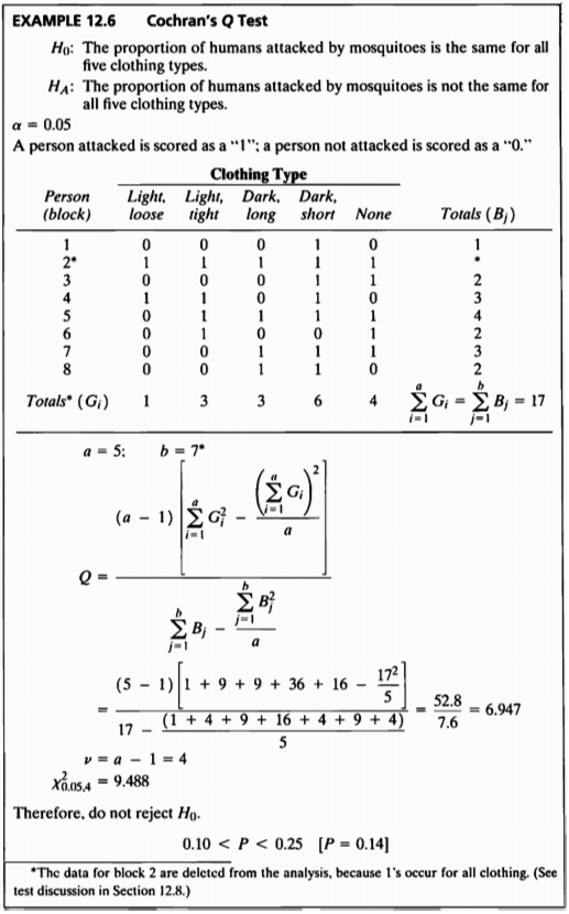
본 데이터는 5가지의 옷에 대해 모기에 공격을 당하는지 안당하는지를 기록한 데이터이다.
Cochran’s Q test는 이항형으로 반복 관측된 데이터에 사용하는 방법으로 이항데이터에 대한 프리드만 검정이라고 할 수 있다.

ex12_6%>%
  kbl(caption = "Dataset of Example 12.2") %>%
  kable_styling(bootstrap_options = c("striped", "hover", "condensed", "responsive"))

Dataset of Example 12.2
exam12_6.Person	exam12_6.Lightloose	exam12_6.Lighttight	exam12_6.Darklong	exam12_6.Darkshort	exam12_6.None
1	0	0	0	1	0
2	1	1	1	1	1
3	0	0	0	1	1
4	1	1	0	1	0
5	0	1	1	1	1
6	0	1	0	0	1
7	0	0	1	1	1
8	0	0	1	1	0

본 검정의 가설은 다음과 같다.

\[\begin{aligned} H_0 &:The\ proportion\ of\ humans\ attacked\ by\ mosquitoes\ is\ the\ same\ for\ all\ five\ clothing\ types.\\ H_A &: The\ proportion\ of\ humans\ attacked\ by\ mosquitoes\ is\ not\ the\ same\ for\ all\ five\ clothing\ types.\\ \end{aligned}\]

Cochran’s Test

library(nonpar)
ex12_6_del <- ex12_6[ex12_6$exam12_6.Person !=2,]
x = ex12_6_del[,-1]
cochrans.q(x)

## 
##  Cochran's Q Test 
##  
##  H0: There is no difference in the effectiveness of treatments. 
##  HA: There is a difference in the effectiveness of treatments. 
##  
##  Q = 6.94736842105263 
##  
##  Degrees of Freedom = 4 
##  
##  Significance Level = 0.05 
##  The p-value is  0.138695841622589 
##   
## 

모든 종류의 옷을 입었을 때 모기에 물린 사람의 데이터는 삭제한다.
Cochran’s Q Test를 수행한 결과, 검정통계량 값은 6.947, p-value는 0.14로 계산되었다.
p-value가 0.05보다 크므로, 유의수준 5%하에 모기의 공격을 받은 사람의 비율은 옷의 종류에 따라 차이가 있다고 결론 내릴 수 없다.

SAS 프로그램 결과

SAS 접기/펼치기 버튼

12장

LIBNAME ex 'C:\Biostat';
RUN;

/*12장 연습문제 불러오기*/
%macro chap09(name=,no=);
%do i=1 %to &no.;
	PROC IMPORT DBMS=excel
		DATAFILE="C:\Biostat\data_chap12"
		OUT=ex.&name.&i. REPLACE;
		RANGE="exam12_&i.$";
	RUN;
%end;
%mend;

%chap09(name=ex12_,no=6);

EXAMPLE 12.1

PROC SORT DATA=ex.ex12_1;
by sex;
run;

PROC MEANS DATA=ex.ex12_1 N Nmiss mean Sum;
class hormone;
by sex;
var plasma_calcium;
run;

PROC MEANS DATA=ex.ex12_1 N Nmiss mean Sum;
var plasma_calcium;
run;

SAS 출력

Example12.6

MEANS 프로시저

Sex=Female


분석 변수: plasma_calcium plasma_calcium
Hormone	관측값 수	N	결측값 수	평균	합계
No Hormone	5	5	0	14.8800000	74.4000000
Yes Hormone	5	5	0	32.5200000	162.6000000

Sex=Male


분석 변수: plasma_calcium plasma_calcium
Hormone	관측값 수	N	결측값 수	평균	합계
No Hormone	5	5	0	12.1200000	60.6000000
Yes Hormone	5	5	0	27.7800000	138.9000000

Example12.6

MEANS 프로시저


분석 변수: plasma_calcium plasma_calcium
N	결측값 수	평균	합계
20	0	21.8250000	436.5000000

EXAMPLE 12.2

/*정규성 검정*/
ods graphics off;ods exclude all;ods noresults;
PROC UNIVARIATE DATA=ex.ex12_1 normal plot;
    CLASS hormone;
    BY sex;
    VAR plasma_calcium;
    ODS OUTPUT TestsForNormality = TestsForNormality;
RUN;
ods graphics on;ods exclude none;ods results;

PROC SORT DATA=TestsForNormality;
    BY descending Test;
RUN;

title " ex12_2 : 정규성 가정";
PROC PRINT DATA=TestsForNormality label; 
    WHERE Test="Shapiro-Wilk"; 
RUN;
title;

/*등분산성 검정*/
ods graphics off;ods exclude all;ods noresults;
PROC GLM DATA=ex.ex12_1;
    CLASS hormone;
    MODEL plasma_calcium=hormone/p;
    MEANS hormone / HOVTEST=BARTLETT;
    ODS OUTPUT Bartlett = Bartlett;
RUN;

PROC GLM DATA=ex.ex12_1;
    CLASS sex;
    MODEL plasma_calcium=sex/p;
    MEANS sex / HOVTEST=BARTLETT;
    ODS OUTPUT Bartlett = Bartlett2;
RUN;
ods graphics on;ods exclude none;ods results;

title "ex12_2 : 등분산 가정 (Bartlett's Test for Homogeneity of weight Variance)";
PROC PRINT DATA=Bartlett label;
RUN;
PROC PRINT DATA=Bartlett2 label;
RUN;
title;

SAS 출력

ex12_2 : 정규성 가정


OBS	Sex	VarName	Hormone	적합도 검정	적합도 통계량에 대한 레이블	적합도 통계량 값	p-값 레이블	p-값
1	Female	plasma_calcium	No Hormone	Shapiro-Wilk	W	0.979256	Pr < W	0.9306
2	Female	plasma_calcium	Yes Hormone	Shapiro-Wilk	W	0.982753	Pr < W	0.9488
3	Male	plasma_calcium	No Hormone	Shapiro-Wilk	W	0.958824	Pr < W	0.7998
4	Male	plasma_calcium	Yes Hormone	Shapiro-Wilk	W	0.978417	Pr < W	0.9260

ex12_2 : 등분산 가정 (Bartlett's Test for Homogeneity of weight Variance)


OBS	Effect	Dependent	Source	DF	Chi-Square	Pr > ChiSq
1	Hormone	plasma_calcium	Hormone	1	0.1999	0.6548

ex12_2 : 등분산 가정 (Bartlett's Test for Homogeneity of weight Variance)


OBS	Effect	Dependent	Source	DF	Chi-Square	Pr > ChiSq
1	Sex	plasma_calcium	Sex	1	0.0915	0.7623

EXAMPLE 12.3

PROC GLM DATA=ex.ex12_1;
    CLASS Hormone sex;
    MODEL plasma_calcium=Hormone sex Hormone*sex;
    LSMEANS  Hormone  sex/diff CL adjust=tukey;
    ODS OUTPUT LSMeanDiffCL=LSMeanDiffCL;
RUN;

SAS 출력

The GLM Procedure


Class Level Information
Class	Levels	Values
Hormone	2	No Hormone Yes Hormone
Sex	2	Female Male


Number of Observations Read	20
Number of Observations Used	20

The GLM Procedure

Dependent Variable: plasma_calcium plasma_calcium


Source	DF	Sum of Squares	Mean Square	F Value	Pr > F
Model	3	1461.325500	487.108500	25.86	<.0001
Error	16	301.392000	18.837000
Corrected Total	19	1762.717500


R-Square	Coeff Var	Root MSE	plasma_calcium Mean
0.829019	19.88619	4.340161	21.82500


Source	DF	Type I SS	Mean Square	F Value	Pr > F
Hormone	1	1386.112500	1386.112500	73.58	<.0001
Sex	1	70.312500	70.312500	3.73	0.0713
Hormone*Sex	1	4.900500	4.900500	0.26	0.6170


Source	DF	Type III SS	Mean Square	F Value	Pr > F
Hormone	1	1386.112500	1386.112500	73.58	<.0001
Sex	1	70.312500	70.312500	3.73	0.0713
Hormone*Sex	1	4.900500	4.900500	0.26	0.6170

Interaction Plot for plasma_calcium by Hormone

The GLM Procedure

Least Squares Means

Adjustment for Multiple Comparisons: Tukey


Hormone	plasma_calcium LSMEAN	H0:LSMean1=LSMean2
Hormone	plasma_calcium LSMEAN	Pr > \|t\|
No Hormone	13.5000000	<.0001
Yes Hormone	30.1500000


Hormone	plasma_calcium LSMEAN	95% Confidence Limits
No Hormone	13.500000	10.590473	16.409527
Yes Hormone	30.150000	27.240473	33.059527


Least Squares Means for Effect Hormone
i	j	Difference Between Means	Simultaneous 95% Confidence Limits for LSMean(i)-LSMean(j)
1	2	-16.650000	-20.764501	-12.535499

Plot of plasma_calcium least-squares means for Hormone.

The GLM Procedure

Least Squares Means

Adjustment for Multiple Comparisons: Tukey


Sex	plasma_calcium LSMEAN	H0:LSMean1=LSMean2
Sex	plasma_calcium LSMEAN	Pr > \|t\|
Female	23.7000000	0.0713
Male	19.9500000


Sex	plasma_calcium LSMEAN	95% Confidence Limits
Female	23.700000	20.790473	26.609527
Male	19.950000	17.040473	22.859527


Least Squares Means for Effect Sex
i	j	Difference Between Means	Simultaneous 95% Confidence Limits for LSMean(i)-LSMean(j)
1	2	3.750000	-0.364501	7.864501

Plot of plasma_calcium least-squares means for Sex.

Plot of all pairwise plasma_calcium least-squares means differences for Sex with Tukey adjustment at significance level 0.05.

PROC PRINT DATA=LSMeanDiffCL;
RUN;

SAS 출력


OBS	Effect	Dependent	i	j	LowerCL	Difference	UpperCL	Hormone	_Hormone	Sex	_Sex
1	Hormone	plasma_calcium	1	2	-20.764501	-16.650000	-12.535499	No Hormone	Yes Hormone
2	Sex	plasma_calcium	1	2	-0.364501	3.750000	7.864501			Female	Male

PROC IML;
    USE ex.ex12_1;
    READ all;
    CLOSE ex.ex12_1;
    female=loc(Sex = "Female");
    male=loc(Sex = "Male");
    total_F = sum(plasma_calcium[female,]);
    total_M = sum(plasma_calcium[male,]);
    number_F = nrow(plasma_calcium[female,]);
    number_M= nrow(plasma_calcium[male,]);
    Xbar_p = round((total_F + total_M) / (number_F + number_M), 0.001);
    t_quantile = round(quantile('T', 1-0.05/2, 16), 0.001);
    s2 = 18.8370;
    margin = t_quantile * sqrt(s2/(number_F+number_M));
    lower_bound = round(Xbar_p - margin, 0.001) ;
    upper_bound = round(Xbar_p + margin, 0.001) ;
*print female male;
*print total_F total_M number_F number_M;
    PRINT Xbar_p lower_bound upper_bound ;
RUN;
QUIT;

SAS 출력

Xbar_p	lower_bound	upper_bound
21.825	19.768	23.882

EXAMPLE 12.4

/*정규성 검정*/
ods graphics off;ods exclude all;ods noresults;
PROC UNIVARIATE DATA=ex.ex12_4 normal plot;
    VAR Time;
    ODS OUTPUT TestsForNormality = TestsForNormality;
RUN;
ods graphics on;ods exclude none;ods results;

PROC SORT DATA=TestsForNormality;
    BY descending Test;
RUN;

title " ex12_2 : 정규성 가정";
PROC PRINT DATA=TestsForNormality label; 
    WHERE Test="Shapiro-Wilk"; 
RUN;
title;

/*등분산성 검정*/
ods graphics off;ods exclude all;ods noresults;
PROC GLM DATA=ex.ex12_4;
    CLASS Treatment;
    MODEL Time=Treatment/p;
    MEANS Treatment / HOVTEST=BARTLETT;
    ODS OUTPUT Bartlett = Bartlett;
RUN;
ods graphics on;ods exclude none;ods results;

title "ex12_2 : 등분산 가정 (Bartlett's Test for Homogeneity of weight Variance)";
PROC PRINT DATA=Bartlett label;
RUN;
title;

SAS 출력

ex12_2 : 정규성 가정


OBS	VarName	적합도 검정	적합도 통계량에 대한 레이블	적합도 통계량 값	p-값 레이블	p-값의 부호	p-값
1	Time	Shapiro-Wilk	W	0.974271	Pr < W		0.9155

ex12_2 : 등분산 가정 (Bartlett's Test for Homogeneity of weight Variance)


OBS	Effect	Dependent	Source	DF	Chi-Square	Pr > ChiSq
1	Treatment	Time	Treatment	2	0.0103	0.9949

ods graphics off;ods exclude all;ods noresults;
PROC GLM DATA=ex.ex12_4;
    CLASS Treatment Block;
    MODEL Time=Treatment Block;
    RANDOM block;
RUN;
ods graphics on;ods exclude none;ods results;

title "Example12.4 ";
ods graphics off;ods exclude all;ods noresults;

PROC GLM DATA=ex.ex12_4 plots=(DIAGNOSTICS RESIDUALS);
    CLASS Treatment Block;
    MODEL Time = Treatment Block;
    RANDOM Block / test;
    ODS OUTPUT OverallANOVA = OverallANOVA_4
    RandomModelANOVA = RandomModelANOVA_4;
RUN;
ods graphics on;ods exclude none;ods results;

PROC PRINT DATA=RandomModelANOVA_4 label;
    VAR Source DF SS MS FValue ProbF;
RUN;

SAS 출력

Example12.4


OBS	Source	DF	Type III SS	Mean Square	F Value	Pr > F
1	Treatment	2	7.708333	3.854167	10.42	0.0059
2	Block	4	11.066667	2.766667	7.48	0.0082
3	Error: MS(Error)	8	2.958333	0.369792	_	_

EXAMPLE 12.5

title "Example12.5 ";
PROC SORT DATA=ex.ex12_4;
    BY block;
RUN;

PROC RANK DATA=ex.ex12_4 out=ex12_4;
   BY Block;
   VAR time;
   RANKS Rtime;
RUN;

PROC PRINT;
   title2 'Original and Ranked Values of Yield';
RUN;

PROC ANOVA DATA=ex12_4;
    CLASS Block Treatment;
    MODEL Rtime = Block Treatment;
    title2 'Friedman''s Two-way Nonparametric ANOVA';
RUN;

SAS 출력

Example12.5

Original and Ranked Values of Yield


OBS	Treatment	Block	Time	Rtime
1	1	1	8.25	1
2	2	1	11.25	3
3	3	1	10.75	2
4	1	2	11.00	1
5	2	2	12.50	3
6	3	2	11.75	2
7	1	3	10.25	1
8	2	3	12.00	3
9	3	3	11.25	2
10	1	4	9.50	2
11	2	4	9.75	3
12	3	4	9.00	1
13	1	5	8.75	1
14	2	5	11.00	3
15	3	5	10.00	2

Example12.5

Friedman's Two-way Nonparametric ANOVA

The ANOVA Procedure


Class Level Information
Class	Levels	Values
Block	5	1 2 3 4 5
Treatment	3	1 2 3


Number of Observations Read	15
Number of Observations Used	15

Example12.5

Friedman's Two-way Nonparametric ANOVA

The ANOVA Procedure

Dependent Variable: Rtime 변수 Time의 순위


Source	DF	Sum of Squares	Mean Square	F Value	Pr > F
Model	6	8.40000000	1.40000000	7.00	0.0075
Error	8	1.60000000	0.20000000
Corrected Total	14	10.00000000


R-Square	Coeff Var	Root MSE	Rtime Mean
0.840000	22.36068	0.447214	2.000000


Source	DF	Anova SS	Mean Square	F Value	Pr > F
Block	4	0.00000000	0.00000000	0.00	1.0000
Treatment	2	8.40000000	4.20000000	21.00	0.0007

EXAMPLE 12.6

title "Example12.6 ";
DATA ex.ex12_6; 
    SET ex.ex12_6;
    IF person=2 THEN delete;
RUN;

ods graphics off;ods exclude all;ods noresults;
PROC FREQ DATA=ex.ex12_6;
    TABLES Lightloose Lighttight Darklong Darkshort None / nocum;
    TABLES Lightloose*Lighttight*Darklong*Darkshort*None / agree noprint;
    ODS OUTPUT CochransQ = CochransQ;
RUN;
ods graphics on;ods exclude none;ods results;

PROC PRINT DATA=CochransQ;
RUN;

SAS 출력

Example12.6


OBS	Table	ChiSquare	DF	Prob
1	Darkshort * None에 대한 요약	6.9474	4	0.1387

교재: Biostatistical Analysis (5th Edition) by Jerrold H. Zar

**이 글은 22학년도 1학기 의학통계방법론 과제 자료들을 정리한 글 입니다.**

Two-Factor Analysis of Variance

R 프로그램 결과

12장

EXAMPLE 12.1

EXAMPLE 12.1a

EXAMPLE 12.2

EXAMPLE 12.2a

EXAMPLE 12.3

EXAMPLE 12.4

EXAMPLE 12.5

EXAMPLE 12.6

SAS 프로그램 결과

12장

EXAMPLE 12.1

EXAMPLE 12.2

EXAMPLE 12.3

EXAMPLE 12.4

EXAMPLE 12.5

EXAMPLE 12.6

Templates (for web app):

Error