[의학통계방법론] Ch11. Multiple Comparisons
Multiple Comparisons
R 프로그램 결과
R 접기/펼치기 버튼
패키지 설치된 패키지 접기/펼치기 버튼
getwd()
## [1] "C:/Biostat"
library("readxl")
library("dplyr")
library("kableExtra")
library("MBESS")
library("DescTools")
library("PMCMRplus")
엑셀파일불러오기
#모든 시트를 하나의 리스트로 불러오는 함수
read_excel_allsheets <- function(file, tibble = FALSE) {
  sheets <- readxl::excel_sheets(file)
  x <- lapply(sheets, function(X) readxl::read_excel(file, sheet = X))
  if(!tibble) x <- lapply(x, as.data.frame)
  names(x) <- sheets
  x
}
11장
11장 연습문제 불러오기
#data_chap11에 연습문제 11장 모든 문제 저장
data_chap11 <- read_excel_allsheets("data_chap11.xls")

#연습문제 각각 데이터 생성
for (x in 1:length(data_chap11)){
  assign(paste0('ex11_',c(1,10))[x],data_chap11[x])
  }

#연습문제 데이터 형식을 리스트에서 데이터프레임으로 변환
for (x in 1:length(data_chap11)){
  assign(paste0('ex11_',c(1,10))[x],data.frame(data_chap11[x]))
  }
EXAMPLE 11.1
#데이터셋
ex11_1%>%
  kbl(caption = "Dataset",escape=F) %>%
  kable_styling(bootstrap_options = c("striped", "hover", "condensed", "responsive"))
| exam11_1.pond | exam11_1.strontium |
|---|---|
| 1 | 28.2 |
| 1 | 33.2 |
| 1 | 36.4 |
| 1 | 34.6 |
| 1 | 29.1 |
| 1 | 31.0 |
| 2 | 39.6 |
| 2 | 40.8 |
| 2 | 37.9 |
| 2 | 37.1 |
| 2 | 43.6 |
| 2 | 42.4 |
| 3 | 46.3 |
| 3 | 42.1 |
| 3 | 43.5 |
| 3 | 48.8 |
| 3 | 43.7 |
| 3 | 40.1 |
| 4 | 41.0 |
| 4 | 44.1 |
| 4 | 46.4 |
| 4 | 40.2 |
| 4 | 38.6 |
| 4 | 36.3 |
| 5 | 56.3 |
| 5 | 54.1 |
| 5 | 59.4 |
| 5 | 62.7 |
| 5 | 60.0 |
| 5 | 57.3 |
- 해당 데이터는 5가지 다른 수역의 strontium 농도(mg/ml) 데이터이다.
- 분산분석을 실시 후 그룹간 차이가 있다는 결론이 났을 때, 어느 그룹간 평균이 차이가 있는지 사후검정을 통해 살펴볼 것이다.
- 이 문제에서는 튜키 검정을 통해 사후검정을 시행해 보았다.
- 우선 분산분석의 가정인 independence, homoscedasticity, normality 살펴보자.
Independence test with residuals
plot(glm(exam11_1.strontium~factor(exam11_1.pond),data=ex11_1)$residual)
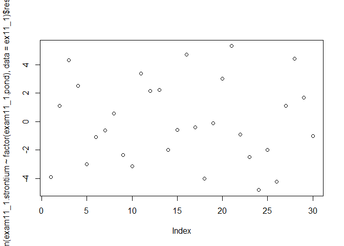
- 잔차에 대한 scatter plot을 봤을 때 골고루 분포 되어 있으므로 독립성을 만족한다 할 수 있다.
Normality test with shapiro test
library(rstatix)
exam11_1.normal<-ex11_1 %>%
  group_by(exam11_1.pond) %>%
  shapiro_test(exam11_1.strontium)

exam11_1.normal %>%
  kbl(caption = "Example11_1 : 정규성 가정") %>%
  kable_styling()
| exam11_1.pond | variable | statistic | p |
|---|---|---|---|
| 1 | exam11_1.strontium | 0.9567420 | 0.7943129 |
| 2 | exam11_1.strontium | 0.9616302 | 0.8322126 |
| 3 | exam11_1.strontium | 0.9718105 | 0.9043687 |
| 4 | exam11_1.strontium | 0.9783967 | 0.9433162 |
| 5 | exam11_1.strontium | 0.9893713 | 0.9875855 |
- 각 수역에서 strontium 농도가 6번씩 측정이 되어 전체 표본의 수는 30이다.
- 표본의 크기가 크지 않으므로 정규성 검정으로 Shapiro-Wilk test를 시행하였으며,
p-value는 각 수역별로 0.7943, 0.8322, 0.9044, 0.9433, 0.9876으로 모두 유의수준 5%하에 귀무가설을 기각할 수 없다. - 따라서 정규성 가정을 만족한다는 귀무가설을 기각할 수 없으므로 정규성 가정을 만족한다고 볼 것이다.
Homoscedasticity test with bartlett test
bartlett.test(ex11_1$exam11_1.strontium,ex11_1$exam11_1.pond)
##
##  Bartlett test of homogeneity of variances
##
## data:  ex11_1$exam11_1.strontium and ex11_1$exam11_1.pond
## Bartlett's K-squared = 0.63895, df = 4, p-value = 0.9586
- 정규성 가정이 모두 만족되었으므로 등분산 검정으로 Bartlett’s Test를 시행하였다.
- p-value는 0.9586으로 유의수준 5%하에 모분산이 서로 동일하다는 귀무가설을 기각하지 못한다.
- 즉, 유의수준 5%하에 등분산 가정을 만족한다고 볼 것이다.
- 분산분석 가정을 모두 만족하였으므로 일원분산분석을 시행하여 보겠다.
ex11_1.anova<-aov(ex11_1$exam11_1.strontium ~ as.factor(ex11_1$exam11_1.pond))
summary(ex11_1.anova)
##                                 Df Sum Sq Mean Sq F value   Pr(>F)
## as.factor(ex11_1$exam11_1.pond)  4 2193.4   548.4   56.16 3.95e-12 ***
## Residuals                       25  244.1     9.8
## ---
## Signif. codes:  0 '***' 0.001 '**' 0.01 '*' 0.05 '.' 0.1 ' ' 1
- 일원분산분석 결과 p-value는 <.0001으로 유의수준 5%하에 귀무가설을 기각한다.
- 유의수준 5%하에 적어도 하나의 수역에서 strontium 농도의 모평균이 다르다고 볼 수 있는 충분한 증거가 있다.
tukey 다중비교
ex11_1.tukey <- TukeyHSD(ex11_1.anova,ordered=T)
ex11_1.tukey$`as.factor(ex11_1$exam11_1.pond)` %>%
  kbl(caption = "Example11_1 : Tukey 다중비교") %>%
  kable_styling()
| diff | lwr | upr | p adj | |
|---|---|---|---|---|
| 2-1 | 8.1500000 | 2.851355 | 13.448645 | 0.0011293 |
| 4-1 | 9.0166667 | 3.718021 | 14.315312 | 0.0003339 |
| 3-1 | 12.0000000 | 6.701355 | 17.298645 | 0.0000053 |
| 5-1 | 26.2166667 | 20.918021 | 31.515312 | 0.0000000 |
| 4-2 | 0.8666667 | -4.431979 | 6.165312 | 0.9884803 |
| 3-2 | 3.8500000 | -1.448645 | 9.148645 | 0.2376217 |
| 5-2 | 18.0666667 | 12.768021 | 23.365312 | 0.0000000 |
| 3-4 | 2.9833333 | -2.315312 | 8.281979 | 0.4791100 |
| 5-4 | 17.2000000 | 11.901355 | 22.498645 | 0.0000000 |
| 5-3 | 14.2166667 | 8.918021 | 19.515312 | 0.0000003 |
plot(ex11_1.tukey, col="forestgreen")

- Appletree Lake-Beaver Lake(4-2), Angler’s Cove-Beaver Lake(3-2), Angler’s Cove-Appletree Lake(3-4) 간에 모평균의 유의한 차이가 없었으며 나머지 수역간에 비교시 유의수준 5% 하에 모평균의 유의한 차이가 있다고 할 수 있다.
EXAMPLE 11.2
ex11_2 <- read_excel(path = 'C:/git_blog/study/data/ch10/data_chap10.xls',sheet = 'exam10_1')
ex11_2[15,3]=NA
ex11_2<-na.omit(ex11_2)
- 독립성, 정규성, 등분산성 가정을 만족함을 Example 10.1에서 이미 확인하였으므로 생략하겠다.
ex11_2.anova <- aov(ex11_2$weight ~ as.factor(ex11_2$diet))
ex11_2.tukey <- TukeyHSD(ex11_2.anova,ordered=T)
ex11_2.tukey$`as.factor(ex11_2$diet)` %>%
  kbl(caption = "Example11_2 : Tukey 다중비교") %>%
  kable_styling()
| diff | lwr | upr | p adj | |
|---|---|---|---|---|
| 1-4 | 1.38 | -4.203737 | 6.963737 | 0.8906642 |
| 2-4 | 8.06 | 2.476263 | 13.643737 | 0.0041505 |
| 3-4 | 10.11 | 4.187553 | 16.032447 | 0.0009497 |
| 2-1 | 6.68 | 1.096263 | 12.263737 | 0.0168421 |
| 3-1 | 8.73 | 2.807553 | 14.652447 | 0.0034914 |
| 3-2 | 2.05 | -3.872447 | 7.972447 | 0.7530266 |
plot(ex11_2.tukey, col = "forestgreen")
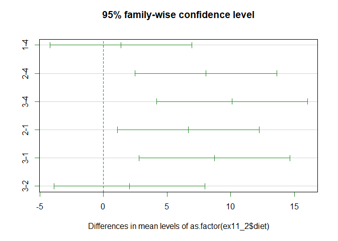
- Feed1-Feed4(1-4), Feed3-Feed2(3-2) 간에 모평균의 유의한 차이가 없었으며 나머지 사료간의 비교시 유의수준 5% 하에 모평균의 유의한 차이가 있다고 할 수 있다.
EXAMPLE 11.3
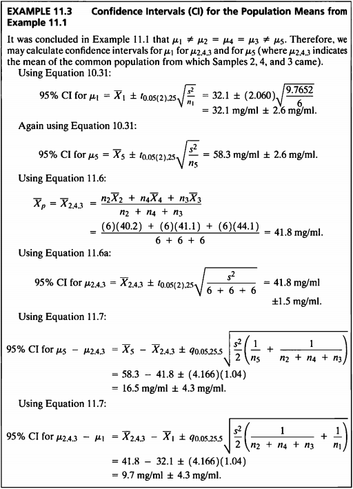
- 이 예제는 Example 11.1 데이터를 사용하여 모평균에 대한 신뢰구간을 구해본다.
library(MBESS)
exam11_1.mean<-aggregate(ex11_1$exam11_1.strontium, by=list(ex11_1$exam11_1.pond), mean)
exam11_1.n <- aggregate(ex11_1$exam11_1.strontium, by=list(ex11_1$exam11_1.pond), length)

ci <- ci.c(means=exam11_1.mean$x, s.anova=sqrt(9.7652),c.weights=c(-3/3,1/3,1/3,1/3,0), n=exam11_1.n$x, N=sum(exam11_1.n$x), conf.level= .95)
data.frame(ci)%>%
  kbl(caption = "CI for the Population Means from ex11_1",escape=F) %>%
  kable_styling(bootstrap_options = c("striped", "hover", "condensed", "responsive"))
| Lower.Conf.Limit.Contrast | Contrast | Upper.Conf.Limit.Contrast |
|---|---|---|
| 6.688301 | 9.722222 | 12.75614 |
- 그룹2,4,3과 그룹1의 모평균 차이의 95% 신뢰구간은 (6.69, 12.76)으로 계산되었다.
ci <- ci.c(means=exam11_1.mean$x, s.anova=sqrt(9.7652),c.weights=c(0,-1/3,-1/3,-1/3,1), n=exam11_1.n$x, N=sum(exam11_1.n$x), conf.level= .95)
data.frame(ci)%>%
  kbl(caption = "CI for the Population Means from ex11_1",escape=F) %>%
  kable_styling(bootstrap_options = c("striped", "hover", "condensed", "responsive"))
| Lower.Conf.Limit.Contrast | Contrast | Upper.Conf.Limit.Contrast |
|---|---|---|
| 13.46052 | 16.49444 | 19.52837 |
- 그룹 5의 모평균과 그룹 2,4,3의 모평균의 차의 95% 신뢰구간은 (13.46, 19.53)으로 계산되었다.
EXAMPLE 11.4
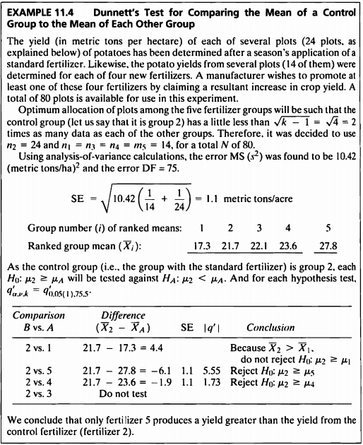
- 해당 데이터는 5가지 비료에 따른 감자 수확량을 mean과 size로 기록한 데이터이다.
mean=c(17.3,21.7,22.1,23.6,27.8)
size= c(14,24,14,14,14)
group=c(1,2,3,4,5)
ex11_4= data.frame(group,mean,size)
ex11_4%>%
  kbl(caption = "Dataset") %>%
  kable_styling(bootstrap_options = c("striped", "hover", "condensed", "responsive"))
| group | mean | size |
|---|---|---|
| 1 | 17.3 | 14 |
| 2 | 21.7 | 24 |
| 3 | 22.1 | 14 |
| 4 | 23.6 | 14 |
| 5 | 27.8 | 14 |
- 기존 2번 비료와 나머지 새로운 비료(1,3,4)를 이용했을 때 감자 수확량의 모평균의 차이가 있는지 확인하기 위해 Dunnett 검정을 사용할 것이다.
Dunnett’s test
k=5
group_index = c(1, 2, 3, 4, 5)
group_n = c(14, 24, 14, 14, 14)
group_mean=c(17.3, 21.7, 22.1, 23.6, 27.8)
N = sum(group_n);
s2 = 10.42;
errorDF=N-k;
se_value = round(sqrt(s2*(1/group_n[1]+1/group_n[2])), 1);
SE = rep(se_value, k)
Difference = rep(group_mean[2], k) - group_mean;
q_prime = abs(round(Difference/se_value, 2));
control = rep(2,k);

exam11_4<-cbind("control"=control, "group_index"=group_index, "Difference"=Difference, "SE"=SE, "q_prime"=q_prime)
exam11_4 %>%
  kbl(caption = "Example11_4 : dunnett") %>%
  kable_styling()
| control | group_index | Difference | SE | q_prime |
|---|---|---|---|---|
| 2 | 1 | 4.4 | 1.1 | 4.00 |
| 2 | 2 | 0.0 | 1.1 | 0.00 |
| 2 | 3 | -0.4 | 1.1 | 0.36 |
| 2 | 4 | -1.9 | 1.1 | 1.73 |
| 2 | 5 | -6.1 | 1.1 | 5.55 |
- 비료 2과 1를 비교한 결과, 표본 평균의 차이가 양수이므로 귀무가설을 기각할 수 없다.
- \(\bar{X}_{2}>\bar{X}_{1}\) 이므로 귀무가설 \(H_{0} : \mu_{2} \geq \mu_{A}\)을 기각할 수 없다.
- 이와 달리 비료 2와 비료 4,5 각각 비교한 결과 표본 평균의 차이가 음수이므로 귀무가설을 기각한다.
- 즉, 기존 2번 비료 보다 새로운 4번 5번 비료를 사용할 때, 감자 수확량의 모평균이 더 크다고 할 수 있다.
- 그룹2와 그룹5를 비교하면 \(\mid q' \mid =5.55\)가 기각역보다 크므로 귀무가설을 기각한다.
- 즉, 유의수준 5%하에서 그룹2의 모평균이 그룹5의 모평균보다 작다고 말할 수 있다.
- 그룹2와 그룹4를 비교하면 \(\mid q' \mid =1.73\)이 기각역보다 크므로 귀무가설을 기각한다.
- 즉, 유의수준 5%하에서 그룹2의 모평균이 그룹5의 모평균보다 작다고 말할 수 있다.
EXAMPLE 11.5
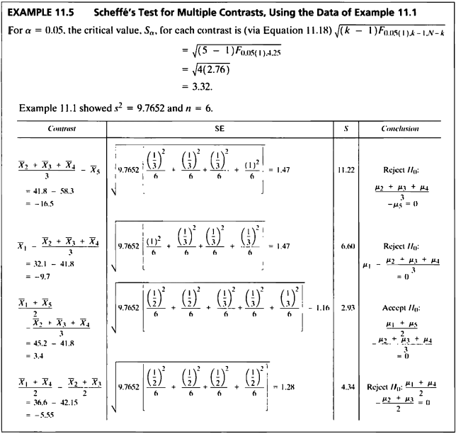
- Dunneet’s test 는 집단과 하나의 control 집단을 이용했다면 Scheffee’s test 에서는 위 문제의 2번 그룹의 대조군과 나머지를 비교하였다.
contrast= matrix(c(0, 1/3, 1/3, 1/3, -1,
                   1, -1/3, -1/3, -1/3, 0,
                   1/2, -1/3, -1/3, -1/3, 1/2,
                   1/2, -1/2, -1/2, 1/2, 0), ncol=4)
library(DescTools)
ex11.6<-ScheffeTest(ex11_1.anova, contrasts=contrast)
ex11.6$`as.factor(ex11_1$exam11_1.pond)` %>%
  kbl(caption = "Example 11.5 & 11.6: SCHEFFE") %>%
  kable_styling()
| diff | lwr.ci | upr.ci | pval | |
|---|---|---|---|---|
| 2,3,4-5 | -16.494444 | -21.3879194 | -11.600969 | 0.0000000 |
| 1-2,3,4 | -9.722222 | -14.6156972 | -4.828747 | 0.0000299 |
| 1,5-2,3,4 | 3.386111 | -0.4825205 | 7.254743 | 0.1090539 |
| 1,4-2,3 | -5.566667 | -9.8045403 | -1.328793 | 0.0054032 |
- 검정 결과 그룹 1,5와 그룹 2,3,4 외에 다른 경우는 유의수준 5%하에 귀무가설을 기각할 충분한 근거를 가지고 있다.
EXAMPLE 11.6
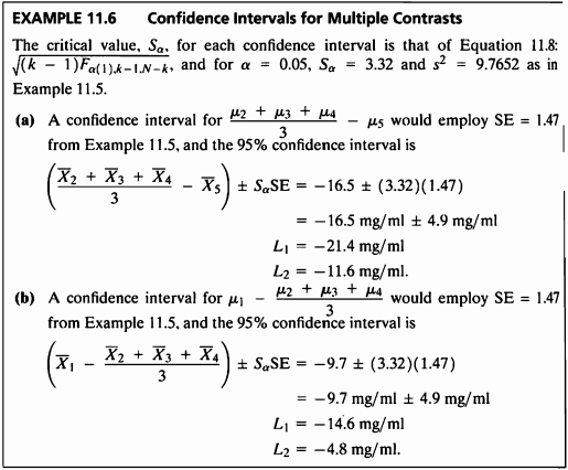
EXAMPLE 11.5 문제의 신뢰구간을 구해본다.
ex11.6$`as.factor(ex11_1$exam11_1.pond)` %>%
  kbl(caption = "Example 11.5 & 11.6: SCHEFFE") %>%
  kable_styling()
- 그룹 (2,3,4)와 그룹 5에 대한 95% 신뢰구간은 (-21.39, -11.60), 그룹 1과 그룹 (2,3,4)에 대한 95% 신뢰구간은 (-14.62,-4.83)이다.
| diff | lwr.ci | upr.ci | pval | |
|---|---|---|---|---|
| 2,3,4-5 | -16.494444 | -21.3879194 | -11.600969 | 0.0000000 |
| 1-2,3,4 | -9.722222 | -14.6156972 | -4.828747 | 0.0000299 |
| 1,5-2,3,4 | 3.386111 | -0.4825205 | 7.254743 | 0.1090539 |
| 1,4-2,3 | -5.566667 | -9.8045403 | -1.328793 | 0.0054032 |
- 그룹 (2,3,4)와 그룹 5에 대한 95% 신뢰구간은 (-21.39, -11.60),
그룹 1과 그룹 (2,3,4)에 대한 95% 신뢰구간은 (-14.62,-4.83)이다.
EXAMPLE 11.7
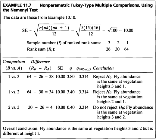
- 이 예제는 EXAMPLE 10.10를 Nemenyi test를 이용하여 비모수적 다중비교를 하는 문제이다.
Nemenyi test
ex11_7 <- read_excel(path = 'C:/git_blog/study/data/ch10/data_chap10.xls',sheet = 'exam10_10')
library(PMCMRplus)
kwAllPairsNemenyiTest(abundance~factor(layer), data=ex11_7, dist='Tukey')
##   1     2
## 2 0.043 -
## 3 0.020 0.957
- PMCMRplus 패키지의 kwAllPairsNemenyiTest() 함수는 Nemenyi test를 이용하여 비모수적인 다중비교 후 p-value를 나타낸 것이다.
- 그룹 1과 2, 그리고 그룹 1과 3간의 비교에서 p-value는 각각 0.043, 0.020으로 유의수준 5%하에서 귀무가설을 기각하였다.
- 그룹 2와 3간의 비교에서 p-value는 0.957이므로 유의수준 5%하에서 귀무가설을 기각하지 못한다.
- 즉, 파리는 2번 식물의 layer와 3번 식물의 layer에서 같지만 1번 식물의 layer에서는 다르다고 할 수 있다.
EXAMPLE 11.8
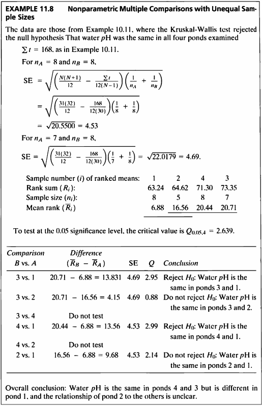
- 이 예제는 EXAMPLE 10.11를 Dunn test를 이용하여 비모수적 다중비교를 하는 문제이다.
- 위 Nemenyi test와 비슷한 방법이지만 표본크기가 다른 데이터이므로 그룹간의 차이가 어떤 그룹간에 있는지 Dunn test를 사용하였다.
Dunn test
ex11_8 <- read_excel(path = 'C:/git_blog/study/data/ch10/data_chap10.xls',sheet = 'exam10_11')
kwAllPairsDunnTest(ex11_8$ph, ex11_8$pond, p.adjust.method = "bonferroni")
##   1     2     3
## 2 0.196 -     -
## 3 0.019 1.000 -
## 4 0.017 1.000 1.000
- 검정 결과 그룹 [1,3], 그룹 [1,4]은 서로 다른 분포를 가지고 있음을 확인할 수 있다.
EXAMPLE 11.9
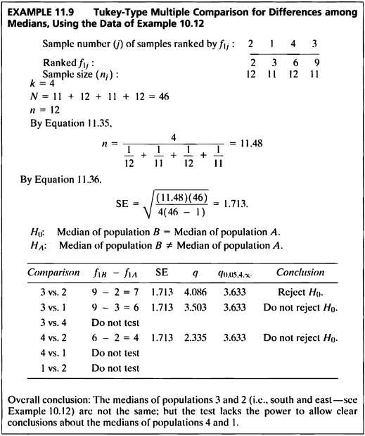
- 이 예제는 EXAMPLE 10.12를 Tukey-Type multiple comparison를 이용하여 그룹간 중앙값의 차이가 있는지 다중비교하는 문제이다.
ex11_9 <- read_excel(path = 'C:/git_blog/study/data/ch10/data_chap10.xls',sheet = 'exam10_12')
median(ex11_9$height)
## [1] 7.9
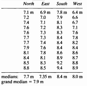
- 중앙값은 7.9 값이 나왔으며, 7.9보다 큰 첫번째 수인 8.1보다 큰 수를 빈도로 잡아 North:3, East:2, South:9, West:6 값이 나온다.
s.size <- c(11,12,11,12)
N <- 46 ; n <- round(4/sum(1/s.size),2) ; se <- round(sqrt(n*N /(4*(N-1))),3)
freq <- c()
for (i in 1:4) {
  freq[i] = length(which(ex11_9$height[ex11_9$side==i] > 8.1))
}
diff <- c(freq[3]-freq[2],freq[3]-freq[1],freq[4]-freq[2])

table <- data.frame(Comparison=c("3 vs. 2", "3 vs. 1", "4 vs. 2"), Difference=diff, SE=se, q= round(diff/se,3), Critical_Value = 3.633)
table %>%
  kbl(caption = "") %>%
  kable_classic(full_width = F, html_font = "Cambria")
| Comparison | Difference | SE | q | Critical_Value |
|---|---|---|---|---|
| 3 vs. 2 | 7 | 1.713 | 4.086 | 3.633 |
| 3 vs. 1 | 6 | 1.713 | 3.503 | 3.633 |
| 4 vs. 2 | 4 | 1.713 | 2.335 | 3.633 |
- 4개의 그룹을 두 그룹 씩 중앙값을 통해 차이 검정을 실시하였다.
- 귀무가설은 ‘두 모집단의 중앙값은 동일하다.’, 대립가설은 ‘두 모집단의 중앙값은 동일하지 않다.’ 이며,
q 통계량이 임계값 3.633 보다 클 경우 귀무가설을 기각한다. - 검정 결과 그룹 3과 2를 비교했을 때, q 통계량이 임계값보다 크므로 귀무가설을 기각하여 3번과 2번 모집단의 중앙값이 서로 동일하지 않음을 알 수 있다.
EXAMPLE 11.10
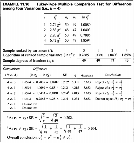
- 이 예제는 분산이 동일하지 않은 결과에 대한 다중비교를 하는 문제이다.
var <- c(2.74,2.83,2.20,6.42) ; n<- c(50,48,50,50) ; v <- n-1 ; treat <- c("1","2","3","4")
q_crit <- 3.633 ; Difference = round(log(c(var[4]/var[3], var[4]/var[1],var[4]/var[2], var[2]/var[3])),4)
SE = round(sqrt(c(1/v[4]+1/v[3], 1/v[4]+1/v[1],1/v[4]+1/v[2],1/v[2]+1/v[3])),3)
table <- data.frame(Comparison=c("4 vs. 3","4 vs. 1","4 vs. 2","2 vs. 3"), Difference,SE, q = round(Difference/SE,3), Critical_Value=q_crit)

table %>%
  kbl(caption = "") %>%
  kable_classic(full_width = F, html_font = "Cambria")
| Comparison | Difference | SE | q | Critical_Value |
|---|---|---|---|---|
| 4 vs. 3 | 1.0710 | 0.202 | 5.302 | 3.633 |
| 4 vs. 1 | 0.8515 | 0.202 | 4.215 | 3.633 |
| 4 vs. 2 | 0.8191 | 0.204 | 4.015 | 3.633 |
| 2 vs. 3 | 0.2518 | 0.204 | 1.234 | 3.633 |
- 4개의 그룹을 두 그룹 씩 등분산 검정을 실시하였다.
- 귀무가설은 ‘두 그룹의 모분산은 동일하다.’, 대립가설은 ‘두 그룹의 모분산은 동일하지 않다.’ 이며,
검정 결과 q 통계량이 임계값 3.633 보다 클 경우 귀무가설을 기각한다. - 검정 결과 그룹 4는 나머지 그룹 전체와 서로 모분산이 동일하지 않으며, 그 외 그룹들의 모분산들은 서로 동일함을 알 수 있다.
SAS 프로그램 결과
SAS 접기/펼치기 버튼
11장
LIBNAME ex 'C:\Biostat';
RUN;

/*11장 연습문제 불러오기*/
%macro chap11(name=,no=);
%do i=1 %to &no.;
	PROC IMPORT DBMS=excel
		DATAFILE="C:\Biostat\data_chap11"
		OUT=ex.&name.&i. REPLACE;
		RANGE="exam11_&i.$";
	RUN;
%end;
%mend;

%chap11(name=ex11_,no=10);
EXAMPLE 11.1
/*정규성 검정*/
ods graphics off;ods exclude all;ods noresults;
PROC UNIVARIATE DATA=ex.ex11_1 normal;
    CLASS pond;
    VAR strontium;
ods output TestsForNormality = TestsForNormality;
RUN;
ods graphics on;ods exclude none;ods results;
PROC SORT DATA=TestsForNormality;
    BY descending Test;
RUN;
title 'ex11_1: 정규성 가정';
PROC PRINT DATA=TestsForNormality label;
RUN;
title;

/*등분산성 검정*/
ods graphics off;ods exclude all;ods noresults;
PROC GLM DATA=ex.ex11_1;
    CLASS pond;
    MODEL strontium= pond/p;
    MEANS pond / HOVTEST=BARTLETT;
    ods output Bartlett = Bartlett;
RUN;
ods graphics on;ods exclude none;ods results;

title "ex11_1 : 등분산 가정 (Bartlett's Test for Homogeneity of weight Variance)";
PROC PRINT DATA=Bartlett label;
RUN;
title;

/*독립성 검정*/
ods graphics off;ods exclude all;ods noresults;
PROC GLM DATA=ex.ex11_1;
    CLASS pond;
    MODEL strontium= pond/p;
    output out=out_ds r=resid_var;
RUN;

DATA out_ds;
    SET out_ds;
        time=_n_;
    ods graphics on;ods exclude none;ods results;
    PROC GPLOT DATA=out_ds;
        PLOT resid_var * time;
RUN;

ods graphics off;ods exclude all;ods noresults;
PROC ANOVA data=ex.ex11_1;
    CLASS pond;
    MODEL strontium=pond;
    MEANS pond /  tukey CLdiff lines;
ods output CLDiffs= CLDiffs_tukey OverallANOVA = OverallANOVA_1;
RUN;
ods graphics on;ods exclude none;ods results;

PROC PRINT DATA=OverallANOVA_1 label;
RUN;

/*다중비교*/
title "ex11.1 : Tukey 다중비교";
PROC SORT DATA=CLDiffs_tukey;
    BY Comparison;
RUN;
PROC PRINT DATA=CLDiffs_tukey label;
    VAR Comparison Difference LowerCL UpperCL Significance;
RUN;
| OBS | VarName | pond | 적합도 검정 | 적합도 통계량에 대한 레이블 | 적합도 통계량 값 | p-값 레이블 | p-값의 부호 | p-값 |
|---|---|---|---|---|---|---|---|---|
| 1 | strontium | 1 | Shapiro-Wilk | W | 0.956742 | Pr < W | 0.7943 | |
| 2 | strontium | 2 | Shapiro-Wilk | W | 0.96163 | Pr < W | 0.8322 | |
| 3 | strontium | 3 | Shapiro-Wilk | W | 0.97181 | Pr < W | 0.9044 | |
| 4 | strontium | 4 | Shapiro-Wilk | W | 0.978396 | Pr < W | 0.9433 | |
| 5 | strontium | 5 | Shapiro-Wilk | W | 0.989372 | Pr < W | 0.9876 | |
| 6 | strontium | 1 | Kolmogorov-Smirnov | D | 0.157345 | Pr > D | > | 0.1500 |
| 7 | strontium | 2 | Kolmogorov-Smirnov | D | 0.155105 | Pr > D | > | 0.1500 |
| 8 | strontium | 3 | Kolmogorov-Smirnov | D | 0.216182 | Pr > D | > | 0.1500 |
| 9 | strontium | 4 | Kolmogorov-Smirnov | D | 0.177547 | Pr > D | > | 0.1500 |
| 10 | strontium | 5 | Kolmogorov-Smirnov | D | 0.141423 | Pr > D | > | 0.1500 |
| 11 | strontium | 1 | Cramer-von Mises | W-Sq | 0.02661 | Pr > W-Sq | > | 0.2500 |
| 12 | strontium | 2 | Cramer-von Mises | W-Sq | 0.0229 | Pr > W-Sq | > | 0.2500 |
| 13 | strontium | 3 | Cramer-von Mises | W-Sq | 0.032535 | Pr > W-Sq | > | 0.2500 |
| 14 | strontium | 4 | Cramer-von Mises | W-Sq | 0.025067 | Pr > W-Sq | > | 0.2500 |
| 15 | strontium | 5 | Cramer-von Mises | W-Sq | 0.0209 | Pr > W-Sq | > | 0.2500 |
| 16 | strontium | 1 | Anderson-Darling | A-Sq | 0.186217 | Pr > A-Sq | > | 0.2500 |
| 17 | strontium | 2 | Anderson-Darling | A-Sq | 0.171671 | Pr > A-Sq | > | 0.2500 |
| 18 | strontium | 3 | Anderson-Darling | A-Sq | 0.195251 | Pr > A-Sq | > | 0.2500 |
| 19 | strontium | 4 | Anderson-Darling | A-Sq | 0.16375 | Pr > A-Sq | > | 0.2500 |
| 20 | strontium | 5 | Anderson-Darling | A-Sq | 0.145265 | Pr > A-Sq | > | 0.2500 |
| OBS | Effect | Dependent | Source | DF | Chi-Square | Pr > ChiSq |
|---|---|---|---|---|---|---|
| 1 | pond | strontium | pond | 4 | 0.6389 | 0.9586 |
| OBS | Dependent | Source | DF | Sum of Squares | Mean Square | F Value | Pr > F |
|---|---|---|---|---|---|---|---|
| 1 | strontium | Model | 4 | 2193.442000 | 548.360500 | 56.15 | <.0001 |
| 2 | strontium | Error | 25 | 244.130000 | 9.765200 | _ | _ |
| 3 | strontium | Corrected Total | 29 | 2437.572000 | _ | _ | _ |
| OBS | pond Comparison | Difference Between Means | LowerCL | UpperCL | Significance |
|---|---|---|---|---|---|
| 1 | 1 - 2 | -8.150 | -13.449 | -2.851 | 1 |
| 2 | 1 - 3 | -12.000 | -17.299 | -6.701 | 1 |
| 3 | 1 - 4 | -9.017 | -14.315 | -3.718 | 1 |
| 4 | 1 - 5 | -26.217 | -31.515 | -20.918 | 1 |
| 5 | 2 - 1 | 8.150 | 2.851 | 13.449 | 1 |
| 6 | 2 - 3 | -3.850 | -9.149 | 1.449 | 0 |
| 7 | 2 - 4 | -0.867 | -6.165 | 4.432 | 0 |
| 8 | 2 - 5 | -18.067 | -23.365 | -12.768 | 1 |
| 9 | 3 - 1 | 12.000 | 6.701 | 17.299 | 1 |
| 10 | 3 - 2 | 3.850 | -1.449 | 9.149 | 0 |
| 11 | 3 - 4 | 2.983 | -2.315 | 8.282 | 0 |
| 12 | 3 - 5 | -14.217 | -19.515 | -8.918 | 1 |
| 13 | 4 - 1 | 9.017 | 3.718 | 14.315 | 1 |
| 14 | 4 - 2 | 0.867 | -4.432 | 6.165 | 0 |
| 15 | 4 - 3 | -2.983 | -8.282 | 2.315 | 0 |
| 16 | 4 - 5 | -17.200 | -22.499 | -11.901 | 1 |
| 17 | 5 - 1 | 26.217 | 20.918 | 31.515 | 1 |
| 18 | 5 - 2 | 18.067 | 12.768 | 23.365 | 1 |
| 19 | 5 - 3 | 14.217 | 8.918 | 19.515 | 1 |
| 20 | 5 - 4 | 17.200 | 11.901 | 22.499 | 1 |
EXAMPLE 11.2
PROC IMPORT DBMS=excel
    DATAFILE="C:\Biostat\data_chap10"
    OUT=ex.ex10_1 REPLACE;
    RANGE="exam10_1$";
RUN;

DATA ex10_1_missing_delte;
     SET ex.ex10_1;
    IF weight=. then delete;
RUN;
ods graphics off;ods exclude all;ods noresults;
PROC ANOVA DATA=ex10_1_missing_delte;
    CLASS diet;
    MODEL weight = diet;
    MEANS diet / TUKEY  cldiff lines;
ods output CLDiffs= CLDiffs_tukey2 OverallANOVA = OverallANOVA_2;
RUN;
ods graphics on;ods exclude none;ods results;

/*분산분석표*/
title "ex11.2 : 분산분석표";
PROC PRINT DATA=OverallANOVA_2 label;
RUN;

PROC SORT DATA=CLDiffs_tukey2;
     BY Comparison;
RUN;
title "ex11.2 : Tukey 다중비교";
PROC PRINT DATA=CLDiffs_tukey2 label;
     VAR Comparison Difference LowerCL UpperCL Significance;
RUN;
| OBS | Dependent | Source | DF | Sum of Squares | Mean Square | F Value | Pr > F |
|---|---|---|---|---|---|---|---|
| 1 | weight | Model | 3 | 338.9373684 | 112.9791228 | 12.04 | 0.0003 |
| 2 | weight | Error | 15 | 140.7500000 | 9.3833333 | _ | _ |
| 3 | weight | Corrected Total | 18 | 479.6873684 | _ | _ | _ |
| OBS | diet Comparison | Difference Between Means | LowerCL | UpperCL | Significance |
|---|---|---|---|---|---|
| 1 | 1 - 2 | -6.680 | -12.264 | -1.096 | 1 |
| 2 | 1 - 3 | -8.730 | -14.652 | -2.808 | 1 |
| 3 | 1 - 4 | 1.380 | -4.204 | 6.964 | 0 |
| 4 | 2 - 1 | 6.680 | 1.096 | 12.264 | 1 |
| 5 | 2 - 3 | -2.050 | -7.972 | 3.872 | 0 |
| 6 | 2 - 4 | 8.060 | 2.476 | 13.644 | 1 |
| 7 | 3 - 1 | 8.730 | 2.808 | 14.652 | 1 |
| 8 | 3 - 2 | 2.050 | -3.872 | 7.972 | 0 |
| 9 | 3 - 4 | 10.110 | 4.188 | 16.032 | 1 |
| 10 | 4 - 1 | -1.380 | -6.964 | 4.204 | 0 |
| 11 | 4 - 2 | -8.060 | -13.644 | -2.476 | 1 |
| 12 | 4 - 3 | -10.110 | -16.032 | -4.188 | 1 |
EXAMPLE 11.3
ods graphics off;ods exclude all;ods noresults;
PROC GLM DATA=ex.ex11_1;
    CLASS pond;
    MODEL strontium = pond/clparm;
    MEANS pond / tukey CLdiff;
    estimate  'pond=1 vs pond=2,3,4'  pond -3 1 1 1 0/divisor=3;
    estimate 'pond=5 vs pond=2,3,4'  pond 0  -1 -1 -1 3/divisor=3;
ods output Estimates=Estimates;
RUN;
QUIT;
ods graphics on;ods exclude none;ods results;

TITLE CI for the Population Means from ex11_1;
PROC PRINT DATA=Estimates;
RUN;
| OBS | Dependent | Parameter | Estimate | StdErr | tValue | Probt | LowerCL | UpperCL |
|---|---|---|---|---|---|---|---|---|
| 1 | strontium | pond=1 vs pond=2,3,4 | 9.7222222 | 1.47310707 | 6.60 | <.0001 | 6.6883014 | 12.7561430 |
| 2 | strontium | pond=5 vs pond=2,3,4 | 16.4944444 | 1.47310707 | 11.20 | <.0001 | 13.4605236 | 19.5283653 |
EXAMPLE 11.4
title "ex11.4: dunnett";
PROC IML;
    k=5;
    group_index = {1 2 3 4 5}`;
    group_n = {14 24 14 14 14}`;
    group_mean={17.3 21.7 22.1 23.6 27.8}`;
    N = sum(group_n);
    s2 = 10.42;
    errorDF=N-k;
    se_value = round(sqrt(s2*(1/group_n[1]+1/group_n[2])), 0.1);
    SE = repeat(se_value, k);
    Difference = repeat(group_mean[2], k) - group_mean;
    q_prime = abs(round(Difference/se_value, 0.01));
    control = repeat(2,k);
create ex.ex11_4 var {control group_index Difference SE q_prime};
    append;
close ex.ex11_4;

PROC PRINT DATA=ex.ex11_4;
    WHERE GROUP_INDEX not in (2 3);
RUN;
| OBS | CONTROL | GROUP_INDEX | DIFFERENCE | SE | Q_PRIME |
|---|---|---|---|---|---|
| 1 | 2 | 1 | 4.4 | 1.1 | 4.00 |
| 4 | 2 | 4 | -1.9 | 1.1 | 1.73 |
| 5 | 2 | 5 | -6.1 | 1.1 | 5.55 |
EXAMPLE 11.5
title "ex11.5 & 11.6: SCHEFFE";
ods graphics off;ods exclude all;ods noresults;
PROC GLM DATA=ex.ex11_1;
    CLASS pond;
    MODEL strontium = pond / solution ss3 CLPARM;
    MEANS pond / SCHEFFE cldiff lines;
    estimate 'pond 234-5' pond 0 1 1 1 -3 / DIVISOR=3;
    estimate 'pond 1-234' pond 3 -1 -1 -1 0 / DIVISOR=3;
    estimate 'pond 15-234' pond 3 -2 -2 -2 3 / DIVISOR=6;
    estimate 'pond 14-23' pond 1 -1 -1 1 0 / DIVISOR=2;
ods output Estimates=Estimates_5;
RUN;
ods graphics on;ods exclude none;ods results;
PROC PRINT DATA=Estimates_5 label;
RUN;
| OBS | Dependent | Parameter | Estimate | Standard Error | t Value | Pr > |t| | LowerCL | UpperCL |
|---|---|---|---|---|---|---|---|---|
| 1 | strontium | pond 234-5 | -16.4944444 | 1.47310707 | -11.20 | <.0001 | -19.5283653 | -13.4605236 |
| 2 | strontium | pond 1-234 | -9.7222222 | 1.47310707 | -6.60 | <.0001 | -12.7561430 | -6.6883014 |
| 3 | strontium | pond 15-234 | 3.3861111 | 1.16459340 | 2.91 | 0.0075 | 0.9875861 | 5.7846361 |
| 4 | strontium | pond 14-23 | -5.5666667 | 1.27574815 | -4.36 | 0.0002 | -8.1941192 | -2.9392142 |
EXAMPLE 11.6
PROC PRINT DATA=Estimates_5 label;
RUN;
| OBS | Dependent | Parameter | Estimate | Standard Error | t Value | Pr > |t| | LowerCL | UpperCL |
|---|---|---|---|---|---|---|---|---|
| 1 | strontium | pond 234-5 | -16.4944444 | 1.47310707 | -11.20 | <.0001 | -19.5283653 | -13.4605236 |
| 2 | strontium | pond 1-234 | -9.7222222 | 1.47310707 | -6.60 | <.0001 | -12.7561430 | -6.6883014 |
| 3 | strontium | pond 15-234 | 3.3861111 | 1.16459340 | 2.91 | 0.0075 | 0.9875861 | 5.7846361 |
| 4 | strontium | pond 14-23 | -5.5666667 | 1.27574815 | -4.36 | 0.0002 | -8.1941192 | -2.9392142 |
EXAMPLE 11.7
%macro KW_MC(source=, groups=, obsname=, gpname=, sig=);
** PERFORM THE STANDARD KRUSKAL WALLIS TEST;
PROC npar1way data=&source wilcoxon;output out=KW_MC_TMP5;
	CLASS &gpname;
	VAR &OBSNAME;
RUN;
* Rank the input data froum the source file;
proc sort data=&source;by &gpname;run;
proc rank data=&source out=KW_MC_TMP6 ties=mean ;
	var &OBSNAME;
	ranks obsrank;
run;
* Determin if there are tied ranks;
proc freq data=KW_MC_TMP6 order=freq ;
	tables obsrank / out=KW_MC_TMP7;
run;
* Create macro variable named &ISTIES;
data _null_;
	if _N_=1 then set KW_MC_TMP7;
	maxtied=count;
	IF MAXTIED gt 1 then TIED=1;ELSE TIED=0;
	CALL SYMPUT('ISTIES',TIED);
run;
* calculate SUMT as per Zar formula 10.42;
proc freq noprint data=KW_MC_TMP6; table obsrank/out=KW_MC_TMP4
	sparse;
run;
data KW_MC_TMP4;set KW_MC_TMP4;
	retain t;
	t=sum(t, (count**3 -count));
	keep t;
run;
data KW_MC_TMP4;
	set KW_MC_TMP4 end=eof;
	N=1;
	if (eof) then output;
run;
*calculate and output the ranksums;
proc means noprint sum n mean data=KW_MC_TMP6;
	output out=rankmeans n=n sum=ranksum mean=rankmean;var
	obsrank;
	by &gpname;
run;
proc sort data=rankmeans;by rankmean;run;
	data rankmeans;set rankmeans;
	label gp ="Rank for Variable &OBSNAME";
run;
data KW_MC_TMP5;set KW_MC_TMP5;
	_label_="Rank for Variable &OBSNAME";
	keep _label_ p_kw;
run;
proc transpose data=rankmeans
	out=KW_MC_TMP5 prefix=MEAN;
	var rankmean;
run;
data KW_MC_TMP5;set KW_MC_TMP5;
	N=_N_;
	keep n mean1-mean&groups;
run;
proc transpose data=rankmeans
	out=KW_MC_TMP6 prefix=n;
	var n;
run;
data KW_MC_TMP6;set KW_MC_TMP6;
	N=_N_;
	keep n n1-n&groups;
run;
proc transpose data=rankmeans
	out=KW_MC_TMP7 prefix=gp;
	var &gpname;
run;
data KW_MC_TMP7;set KW_MC_TMP7;
	N=_N_;
	keep n gp1-gp&groups;
run;
data transposed;
	merge KW_MC_TMP5 KW_MC_TMP6 KW_MC_TMP7 KW_MC_TMP4;
	by n;
run;
data tmp4;set transposed;
	format msg $53.;
	sumt=t;
	iputrejectmessage=0;
	msg="Do not test";*set length of variable;
	msg="Reject";
	array ranksum(*) mean1-mean&groups;
	array na(*) n1-n&groups;
	array lab(*) gp1-gp&groups;
	array q05(20);
	array pair(20,20);
* Check to see if all group ns are equal;
notequal=0;
		do i=1 to &groups ;
		if na(1) ne na(i) then notequal=1;
		end;
* if there are ties, use the notequal version of the comparisons;
tmp=&isties;
if tmp eq 1 then notequal=1;
ALPHA=&sig;
Q05(1)=.;
		do K=2 to 20;
		PQ=1-ALPHA/(K*(k-1));
		Q05(K)=PROBIT(PQ);
		end;
xx= Q05(3);
if notequal=0 then
		do K=2 to 20;
		PQ =1-ALPHA;
		q05(k)=probmc("RANGE", .,PQ,64000,k);
		end;
nsum=0;
		do i=1 to &groups;
		nsum=nsum+na(i);
		end;
icompare=&groups;
qcrit=q05(icompare);
* print out the multiple comparison results table;
file print;
gp="&gpname";
if notequal=1 then
	do;
	put @5 "Group sample sizes not equal, or some ranks tied. Performed Dunn's test, alpha="
	alpha;
	end;
	else do ;
	put @5 "Group sample sizes are equal. Performed Nemenyi test, alpha="
    alpha;
	end;
	put ' ';
	put @5 'Comparison group = ' "&gpname";
	put ' ';
	put ' Compare Diff SE q q(' "&sig" ') Conclude';
	put '------------------------------------------------------------';
iskiprest=0;
* as the table is constructed, determine the correct Conclude message;
	do i=icompare to 1 by -1;
	do j=1 to i;
	pair(i,j)=0; *0=not yet tested, 1=reject 2=accept 3= skip;
	end;
	end;
	do i=icompare to 1 by -1;
	do j=1 to i;
	if i ne j then do;
	if notequal=0 then
	do;
	* Zar formula 11.22;
	rs1=ranksum(i)*na(1);
	rs2=ranksum(j)*na(1);
	se=round(sqrt((na(1)*(na(1)*&groups)*(na(1)*&groups+1))/12),.01)
	;
	end;
	else do;
rs1=ranksum(i);
rs2=ranksum(j);
	* Zar formula 11.28;
	setmp=( ((nsum*(nsum+1))/12) -(SUMT/
	(12*(nsum-1)) ))*( (1/na(i))+ (1/na(j)) );
	se=round(sqrt(setmp),.01);
	end;
diff=round(rs1-rs2,.01);
q=round((rs1-rs2)/se,.01);
	if pair(i,j) ne 3 then do;
	if (q gt qcrit) and (pair(i,j) ne 2) then
	pair(i,j)=1; * REJECT;
	if q le qcrit then do;
	pair(i,j)=2;
	if (i-j) ge 2 then do;
	do k=j to (i-1); do l=(k+1) to i;
	if icompare ne 1 then do;
	if (pair(l,k) ne 2) and
	(l ne k) then pair(l,k)=3;* set to not test;
	end;
	end;
	end;
	end;
	end;
	end;
if pair(i,j)=1 then msg='Reject';
if pair(i,j)=2 then msg='Do not reject';
if pair(i,j)=3 then msg='Do not reject
(within non-sig. comparison)';
	if pair(i,j)=3 then iputrejectmessage=1;
	if pair(i,j) le 2 then
	put @5 lab(i) 'vs' @11 lab(j) @ 15 diff @25 se
	@35 q @45 qcrit 6.3 @55 msg ;
	if pair(i,j)=3 then
	put @5 lab(i) 'vs' @11 lab(j) @15 msg;
	end;
	end;
	end;
	if iputrejectmessage=1 then do;
	put ' ';
	put ' Note: "Do not reject (within non-sig.comparison)" indicates that any comparison';
	put ' within the range of a non-significant comparison must also be non-significant.';
	end;
put ' ';
put ' Reference: Biostatistical Analysis, 4th Edition, J. Zar, 2010.';
run;
%mend KW_MC;
%KW_MC(source=ex.ex10_10, groups=3, obsname=abundance, gpname=layer, sig=0.05);
The NPAR1WAY Procedure
| Wilcoxon Scores (Rank Sums) for Variable abundance Classified by Variable layer | |||||
|---|---|---|---|---|---|
| layer | N | Sum of Scores | Expected Under H0 | Std Dev Under H0 | Mean Score |
| 1 | 5 | 64.0 | 40.0 | 8.164966 | 12.80 |
| 2 | 5 | 30.0 | 40.0 | 8.164966 | 6.00 |
| 3 | 5 | 26.0 | 40.0 | 8.164966 | 5.20 |
| Kruskal-Wallis Test | ||
|---|---|---|
| Chi-Square | DF | Pr > ChiSq |
| 8.7200 | 2 | 0.0128 |

FREQ 프로시저
| 변수 abundance의 순위 | ||||
|---|---|---|---|---|
| obsrank | 빈도 | 백분율 | 누적 빈도 | 누적 백분율 |
| 1 | 1 | 6.67 | 1 | 6.67 |
| 2 | 1 | 6.67 | 2 | 13.33 |
| 3 | 1 | 6.67 | 3 | 20.00 |
| 4 | 1 | 6.67 | 4 | 26.67 |
| 5 | 1 | 6.67 | 5 | 33.33 |
| 6 | 1 | 6.67 | 6 | 40.00 |
| 7 | 1 | 6.67 | 7 | 46.67 |
| 8 | 1 | 6.67 | 8 | 53.33 |
| 9 | 1 | 6.67 | 9 | 60.00 |
| 10 | 1 | 6.67 | 10 | 66.67 |
| 11 | 1 | 6.67 | 11 | 73.33 |
| 12 | 1 | 6.67 | 12 | 80.00 |
| 13 | 1 | 6.67 | 13 | 86.67 |
| 14 | 1 | 6.67 | 14 | 93.33 |
| 15 | 1 | 6.67 | 15 | 100.00 |
    Group sample sizes are equal. Performed Nemenyi test, alpha=0.05
    Comparison group = layer
 Compare Diff SE q q(0.05) Conclude
------------------------------------------------------------
    1 vs  3   38        10        3.8        3.315    Reject
    1 vs  2   34        10        3.4        3.315    Reject
    2 vs  3   4         10        0.4        3.315    Do not reject
 Reference: Biostatistical Analysis, 4th Edition, J. Zar, 2010.
EXAMPLE 11.8
PROC IMPORT DBMS=excel
    DATAFILE="C:\Biostat\data_chap10"
    OUT=ex.ex10_11 REPLACE;
    RANGE="exam10_11$";
RUN;

%LET NUMGROUPS=4;
%LET DATANAME=ex.ex10_11;
%LET OBSVAR=ph;
%LET GROUP=pond;
%LET ALPHA=0.05;
* OPTINALLY DEFINE A TITLE;
TITLE 'Kruskal-Wallis Tied Ranks';
RUN;

ODS HTML;
%KW_MC(source=&DATANAME, groups=&NUMGROUPS, obsname=&OBSVAR, gpname=&GROUP, sig=&alpha);
ODS HTML CLOSE;
The NPAR1WAY Procedure
| Wilcoxon Scores (Rank Sums) for Variable ph Classified by Variable pond | |||||
|---|---|---|---|---|---|
| pond | N | Sum of Scores | Expected Under H0 | Std Dev Under H0 | Mean Score |
| Average scores were used for ties. | |||||
| 1 | 8 | 55.00 | 128.0 | 22.088386 | 6.875000 |
| 2 | 8 | 132.50 | 128.0 | 22.088386 | 16.562500 |
| 3 | 7 | 145.00 | 112.0 | 21.106183 | 20.714286 |
| 4 | 8 | 163.50 | 128.0 | 22.088386 | 20.437500 |
| Kruskal-Wallis Test | ||
|---|---|---|
| Chi-Square | DF | Pr > ChiSq |
| 11.9435 | 3 | 0.0076 |

FREQ 프로시저
| 변수 ph의 순위 | ||||
|---|---|---|---|---|
| obsrank | 빈도 | 백분율 | 누적 빈도 | 누적 백분율 |
| 13.5 | 4 | 12.90 | 4 | 12.90 |
| 6 | 3 | 9.68 | 7 | 22.58 |
| 10 | 3 | 9.68 | 10 | 32.26 |
| 20 | 3 | 9.68 | 13 | 41.94 |
| 26 | 3 | 9.68 | 16 | 51.61 |
| 3.5 | 2 | 6.45 | 18 | 58.06 |
| 23.5 | 2 | 6.45 | 20 | 64.52 |
| 1 | 1 | 3.23 | 21 | 67.74 |
| 2 | 1 | 3.23 | 22 | 70.97 |
| 8 | 1 | 3.23 | 23 | 74.19 |
| 16 | 1 | 3.23 | 24 | 77.42 |
| 17 | 1 | 3.23 | 25 | 80.65 |
| 18 | 1 | 3.23 | 26 | 83.87 |
| 22 | 1 | 3.23 | 27 | 87.10 |
| 28 | 1 | 3.23 | 28 | 90.32 |
| 29 | 1 | 3.23 | 29 | 93.55 |
| 30 | 1 | 3.23 | 30 | 96.77 |
| 31 | 1 | 3.23 | 31 | 100.00 |
    Group sample sizes not equal, or some ranks tied. Performed Dunn's test, alpha=0.05
    Comparison group = pond
 Compare Diff SE q q(0.05) Conclude
------------------------------------------------------------
    3 vs  1   13.84     4.69      2.95       2.638    Reject
    3 vs  2   4.15      4.69      0.89       2.638    Do not reject
    3 vs  4   Do not reject(within non-sig. comparison)
    4 vs  1   13.56     4.53      2.99       2.638    Reject
    4 vs  2   Do not reject(within non-sig. comparison)
    2 vs  1   9.69      4.53      2.14       2.638    Do not reject
 Note: "Do not reject (within non-sig.comparison)" indicates that any comparison
 within the range of a non-significant comparison must also be non-significant.
 Reference: Biostatistical Analysis, 4th Edition, J. Zar, 2010.
EXAMPLE 11.9
%macro ex11_9(a,b);
proc iml;
	f={12,11,12,11};
	n=4/(1/12+1/11+1/12+1/11);
	se=sqrt((11.48*sum(f))/(4*(sum(f)-1)));
	q=(&b-&a)/se;
	print q;run;quit;
	%mend;
TITLE '3 vs 2';
	%ex11_9(2,9);
TITLE '3 vs 1';
	%ex11_9(3,9);
TITLE '4 vs 2';
	%ex11_9(2,6);
| q |
|---|
| 4.0868099 |
| q |
|---|
| 3.5029799 |
| q |
|---|
| 2.3353199 |
EXAMPLE 11.10
%macro ex11_10(n1_a,n2_a,s1_a,s2_a);
proc iml;
	se=sqrt(1/(&n1_a-1)+1/(&n2_a-1));
	q=(log(&s1_a)-log(&s2_a))/se;
	print se q;run;quit;
	%mend;
TITLE '4 vs 3';
	%ex11_10(50,50,6.42,2.20);
TITLE '4 vs 1';
	%ex11_10(50,50,6.42,2.74);
TITLE '4 vs 2';
	%ex11_10(50,48,6.42,2.83);
TITLE '2 vs 3';
	%ex11_10(48,50,2.83,2.20);
| se | q |
|---|---|
| 0.2020305 | 5.3009853 |
| se | q |
|---|---|
| 0.2020305 | 4.214513 |
| se | q |
|---|---|
| 0.2041685 | 4.012086 |
| se | q |
|---|---|
| 0.2041685 | 1.2333901 |
교재: Biostatistical Analysis (5th Edition) by Jerrold H. Zar
**이 글은 22학년도 1학기 의학통계방법론 과제 자료들을 정리한 글 입니다.**