[의학통계방법론] Ch10. Multisample Hypotheses and the Analysis of Variance

07 Apr 2022 in Study log / Study / 의학통계방법론 on R, Sas, Blog, Jekyll, Jupyter, Data, Python

Multisample Hypotheses and
the Analysis of Variance
R 프로그램 결과
- 10장
SAS 프로그램 결과
- 10장

Multisample Hypotheses and
the Analysis of Variance

예제 데이터파일 다운로드

R 프로그램 결과

R 접기/펼치기 버튼

패키지

설치된 패키지 접기/펼치기 버튼

getwd()

## [1] "C:/Biostat"

library("readxl")
library("dplyr")
library("kableExtra")
library("randtests")
library("lmtest")
library("car")
library("lawstat")
library("onewaytests")
library("pwr2")
library("pgirmess")
library("DescTools")
library("RVAideMemoire")

엑셀파일불러오기

#모든 시트를 하나의 리스트로 불러오는 함수
read_excel_allsheets <- function(file, tibble = FALSE) {
  sheets <- readxl::excel_sheets(file)
  x <- lapply(sheets, function(X) readxl::read_excel(file, sheet = X, na = "."))
  if(!tibble) x <- lapply(x, as.data.frame)
  names(x) <- sheets
  x
}

10장

10장 연습문제 불러오기

#data_chap10에 연습문제 10장 모든 문제 저장
data_chap10 <- read_excel_allsheets("data_chap10.xls")

#연습문제 각각 데이터 생성
for (x in 1:length(data_chap10)){
  assign(paste0('ex10_',c(1:3,10:13))[x],data_chap10[x])
  }

#연습문제 데이터 형식을 리스트에서 데이터프레임으로 변환
for (x in 1:length(data_chap10)){
  assign(paste0('ex10_',c(1:3,10:13))[x],data.frame(data_chap10[x]))
  }

EXAMPLE 10.1

#데이터셋
ex10_1%>%
  kbl(caption = "Dataset",escape=F) %>%
  kable_styling(bootstrap_options = c("striped", "hover", "condensed", "responsive"))

Dataset
exam10_1.id	exam10_1.diet	exam10_1.weight
1	1	60.8
2	1	67.0
3	1	65.0
4	1	68.6
5	1	61.7
6	2	68.7
7	2	67.7
8	2	75.0
9	2	73.3
10	2	71.8
11	3	69.6
12	3	77.1
13	3	75.2
14	3	71.5
15	3	NA
16	4	61.9
17	4	64.2
18	4	63.1
19	4	66.7
20	4	60.3

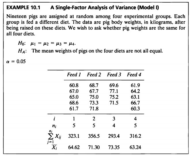
데이터: 19마리 돼지를 4개 그룹으로 무작위로 나누어 서로 다른 다이어트 처리 후 중량(kg) 측정

이 문제의 데이터는 돼지의 체중(weight) 증가에 가장 효율적인 사료(feed)를 찾기 위한 실험에서 얻어진 측정값들이다.
19마리의 돼지가 각 처리별로 랜덤배정되었다.
사료의 종류에 따라 나뉘어진 네 집단 간 무게의 모평균에 차이가 있는지를 검정할 것이다.

\[\begin{aligned} H_0&:\ \mu_1=\mu_2=\mu_3=\mu_4.\\ H_A&:\ The\ mean\ weights\ of\ pigs\ on\ the\ four\ diets\ are\ not\ all\ equal.\\ \end{aligned}\]

단일 요인 분산 분석 ANOVA는 완전히 랜덤화 된 실험 설계 방법이다.
“completely randomized design”이라고도 한다.
일반적으로 데이터에서 그룹의 통계적 비교는 각 그룹의 데이터 수가 동일한 경우(균형적인 상황)에 가장 적합하다.
균형적일 때 검정의 검정력이 높아진다.
하지만 10.1의 데이터의 경우 4개의 그룹 각각에 5마리의 실험동물이 있지만,
Feed 3에 속한 한 마리의 동물의 몸무게는 어떤 적절한 이유로 분석에 사용되지 않았다.
아니면 병이 났거나 임신한 것으로 밝혀졌을 수도 있다.
분산 분석에서는 실험 요인을 제외한 모든 면에서 가능한 유사해야 한다.
(즉, 동물은 동일한 품종, 성별, 연령이어야 하고, 같은 온도로 유지되어야 한다.)

분석을 위한 통계량

ex10_1 %>% 
  group_by(exam10_1.diet) %>% 
  summarize(mean=mean(exam10_1.weight,na.rm=T),sum=sum(exam10_1.weight,na.rm=T))%>%
  kbl(caption = "Dataset") %>%
  kable_styling(bootstrap_options = c("striped", "hover", "condensed", "responsive"))

Dataset
exam10_1.diet	mean	sum
1	64.62	323.1
2	71.30	356.5
3	73.35	293.4
4	63.24	316.2

EXAMPLE 10.1a

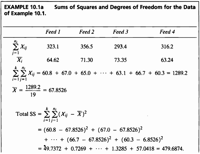
분석을 위해 결측치 제거해준 뒤 자유도와 제곱합들을 구하도록 한다.

ex10_1[15,3]=NA
ex10_1<-na.omit(ex10_1)

ex10_1a <- function(x){
  sum <- ex10_1 %>% summarize(sum=sum(exam10_1.weight,na.rm=T))
  mean <- ex10_1 %>% summarize(mean=mean(exam10_1.weight,na.rm=T))
  total_df<-length(x)-1
  groups_df<-length(unique(ex10_1$exam10_1.diet))-1
  error_df<-length(x)-length(unique(ex10_1$exam10_1.diet))
  y <- rep(0,4)
  for (i in 1:4){
    y[i]=length(ex10_1[ex10_1$exam10_1.diet==i,3])*((mean(ex10_1[ex10_1$exam10_1.diet==i,3])-mean(x))^2)
  }
  SSB=sum(y)
  SST=sum((x-mean(x))^2)
  SSE=SST-SSB
  table <- data.frame(total_DF=total_df,groups_DF=groups_df,error_DF=error_df,Total_SS=SST,Group_SS=SSB,Error_SS=SSE)
  return(table)
}

ex10_1a(ex10_1$exam10_1.weight)%>%
  kbl(caption = "Dataset",escape=F) %>%
  kable_styling(bootstrap_options = c("striped", "hover", "condensed", "responsive"))

Dataset
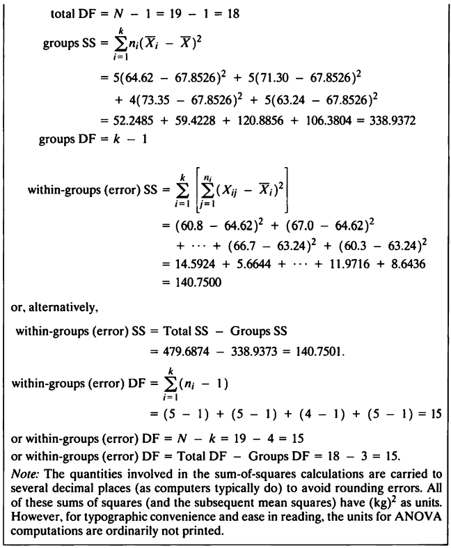
total_DF	groups_DF	error_DF	Total_SS	Group_SS	Error_SS
18	3	15	479.6874	338.9374	140.75

EXAMPLE 10.1b

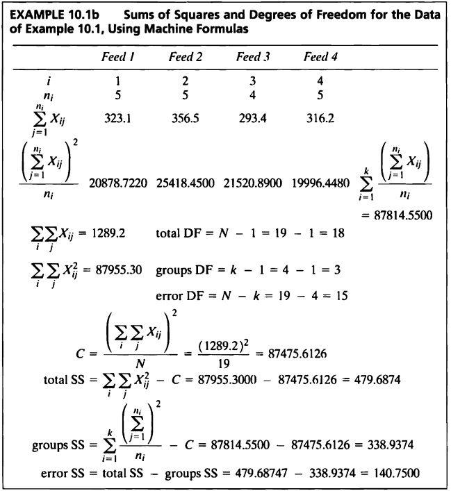
“Machine Formulas”라는 새로운 방식을 사용한 결과는 다음과 같다.

\[\begin{aligned} Total\ SS&=\sum_{i=1}^k\ \sum_{j=1}^{n_i}X_{ij}^2-C\\\\ group\ SS&=\sum_{i=1}^k \frac{(\sum_{j=1}^{n_i}X_{ij})^2}{n_i}-C\\\\ error\ SS&=\sum_{i=1}^k\ \sum_{j=1}^{n_i}X_{ij}^2-\sum_{i=1}^k \frac{(\sum_{j=1}^{n_i}X_{ij})^2}{n_i}\\\\ where\ C&=\frac{(\sum_{i} \sum_{j} \ X_{ij})^2}{N} \end{aligned}\]

ex10_1b <- function(){
  sum <- ex10_1 %>% summarize(sum=sum(exam10_1.weight,na.rm=T))
  sum_s <- ex10_1 %>% summarize(sum_s=sum((exam10_1.weight)^2,na.rm=T))
  c <- sum^2/length(ex10_1$exam10_1.weight)
  y <- rep(0,4)
  for (i in 1:4){
    y[i]=(sum(ex10_1[ex10_1$exam10_1.diet==i,3])^2)/(length(ex10_1[ex10_1$exam10_1.diet==i,3]))
  }
  ss <- sum(y)
  tss <- round(sum_s-c,4)
  gss <- (ss-c)
  ess <- (round(sum_s-c,4)-(ss-c))
  table <- data.frame(tss,gss,ess)
  names(table) <- c("Total_SS","Group_SS","Error_SS")
  return(table)
}

ex10_1b()%>%
  kbl(caption = "Dataset",escape=F) %>%
  kable_styling(bootstrap_options = c("striped", "hover", "condensed", "responsive"))

Dataset
Total_SS	Group_SS	Error_SS
479.6874	338.9374	140.75

“Machine Formulas” 방법을 사용한 결과와 10.1a에서 구한 결과가 같은 것을 확인할 수 있다.
예제 10.1b와 같이 간단한 계산기를 사용할 때 이와 같은 기계식은 매우 편리할 수 있지만, 통계적 계산을 컴퓨터에 의해 수행하는 경우에는 덜 중요하다.

EXAMPLE 10.1c

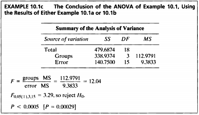
10.1a와 10.1b에서 구한 값들을 토대로 ANOVA를 진행하도록 한다.
일원분산분석을 진행하기 전에 정규성과 등분산성, 독립성을 만족하는지 부터 확인하도록 한다.

Shapiro-Wilk Test로 네 그룹의 정규성을 평가하였다.

shapiro.test(subset(ex10_1$exam10_1.weight,ex10_1$exam10_1.diet==1));shapiro.test(subset(ex10_1$exam10_1.weight,ex10_1$exam10_1.diet==2));shapiro.test(subset(ex10_1$exam10_1.weight,ex10_1$exam10_1.diet==3));shapiro.test(subset(ex10_1$exam10_1.weight,ex10_1$exam10_1.diet==4))  

## 
##  Shapiro-Wilk normality test
## 
## data:  subset(ex10_1$exam10_1.weight, ex10_1$exam10_1.diet == 1)
## W = 0.93315, p-value = 0.618

## 
##  Shapiro-Wilk normality test
## 
## data:  subset(ex10_1$exam10_1.weight, ex10_1$exam10_1.diet == 2)
## W = 0.94389, p-value = 0.6936

## 
##  Shapiro-Wilk normality test
## 
## data:  subset(ex10_1$exam10_1.weight, ex10_1$exam10_1.diet == 3)
## W = 0.95202, p-value = 0.7287

## 
##  Shapiro-Wilk normality test
## 
## data:  subset(ex10_1$exam10_1.weight, ex10_1$exam10_1.diet == 4)
## W = 0.99027, p-value = 0.9806

네 그룹 모두 정규성 검정 결과 p-value가 0.05보다 매우 크므로 네 그룹 모두 모집단이 정규성을 따르지 않는다는 대립가설을 채택할 충분한 근거가 없다.
따라서 정규성을 만족한다는 사실을 바탕으로 그룹별 등분산성 검정을 진행한다.

Bartlett’s Test를 통해 네 그룹의 등분산성 검정을 진행하였다.

bartlett.test(ex10_1$exam10_1.weight~ex10_1$exam10_1.diet)

## 
##  Bartlett test of homogeneity of variances
## 
## data:  ex10_1$exam10_1.weight by ex10_1$exam10_1.diet
## Bartlett's K-squared = 0.47515, df = 3, p-value = 0.9243

Bartlett’s Test의 유의확률은 p-value = 0.9243으로 유의수준 0.05보다 매우 크므로 등분산성이 아니라는 대립가설을 채택할 근거가 없다.
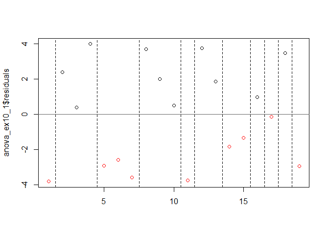
Runs Test와 Durbin-Watson test을 통하여 잔차의 자기상관성을 확인하여 보겠다.

Runs Test

anova_ex10_1 <- aov(ex10_1$exam10_1.weight~as.factor(ex10_1$exam10_1.diet))
library(randtests)
runs.test(anova_ex10_1$residuals, alternative = "two.sided", threshold = 0.0, plot = TRUE)

## 
##  Runs Test - Two sided
## 
## data:  anova_ex10_1$residuals
## Standardized Runs Statistic = 0.24922, p-value = 0.8032

잔차 그림을 확인하여 보면 뚜렷한 패턴이 보이지 않았다.
Runs Test의 경우 양의 계열상관을 검정하기 위해서는 하한임계치를 사용하고,
음의 계열상관을 검정하기 위해서는 상한 임계치를 사용하며, 계열상관의 존재 여부를 위해서는 양쪽 임계치 모두를 사용한다.
양측 검정을 시행하였으며, p-value = 0.8032이므로 귀무가설 “연속적인 관측값이 임의적이다.”를 기각하지 못한다.

Durbin-Watson test

library(lmtest)
dwtest(anova_ex10_1, alternative = "greater")

## 
##  Durbin-Watson test
## 
## data:  anova_ex10_1
## DW = 2.2368, p-value = 0.4203
## alternative hypothesis: true autocorrelation is greater than 0

Durbin-Watson test의 경우 DW = 2.2368으로 4보다 2와 가깝게 나왔으며, 2보다 크므로 alternative = “greater” 주었고 p-value = 0.4203으로 귀무가설 “자기상관이 0 이다.”를 기각하지 못한다.
자기상관성이 없다고 독립인 건 아니지만 독립성 가정이 만족된다고 가정할 수 있을 것 같다.
Shapiro-Wilk test와 Bartlett’s Test으로 정규성과 등분산성을 확인하였으므로 ANOVA 검정을 진행한다.

class(ex10_1$exam10_1.diet)

## [1] "numeric"

diet의 class가 numeric이므로 factor로 변경해서 ANOVA 검정을 실시한다.

summary(aov(ex10_1$exam10_1.weight~as.factor(ex10_1$exam10_1.diet)))

##                                 Df Sum Sq Mean Sq F value   Pr(>F)    
## as.factor(ex10_1$exam10_1.diet)  3  338.9  112.98   12.04 0.000283 ***
## Residuals                       15  140.8    9.38                     
## ---
## Signif. codes:  0 '***' 0.001 '**' 0.01 '*' 0.05 '.' 0.1 ' ' 1

p-value가 0.000283으로 유의수준 0.05보다 매우 작기 때문에 귀무가설을 기각할 수 있고 따라서 유의수준 5%하에 식단에 따른 돼지의 몸무게 모평균 차이가 있다고 말할 수 있다.

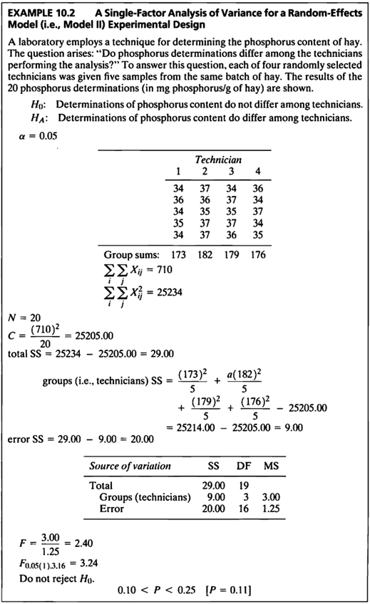
EXAMPLE 10.2

#데이터셋
ex10_2

##    exam10_2.id exam10_2.technician exam10_2.phosphorus
## 1            1                   1                  34
## 2            2                   1                  36
## 3            3                   1                  34
## 4            4                   1                  35
## 5            5                   1                  34
## 6            6                   2                  37
## 7            7                   2                  36
## 8            8                   2                  35
## 9            9                   2                  37
## 10          10                   2                  37
## 11          11                   3                  34
## 12          12                   3                  37
## 13          13                   3                  35
## 14          14                   3                  37
## 15          15                   3                  36
## 16          16                   4                  36
## 17          17                   4                  34
## 18          18                   4                  37
## 19          19                   4                  34
## 20          20                   4                  35

실험실에서 건초의 인 함량을 측정하는 기술을 사용하는데
“인 측정값이 분석을 수행하는 기술자마다 다릅니까?”라는 질문이 발생한다.
이 질문에 답하기 위해 무작위로 선택된 네 명의 기술자 각각에게 동일한 건초 배치에서 5개의 샘플이 주어졌고, 20개의 인 측정 결과(건초 mg/g)가 표시된다.
Example 10.2는 랜덤 효과 모형에 대한 분산 분석을 보여준다.
Example 10.2의 심각한 결과는 기본 가정으로부터 이탈하는 경우이다.
다행히도 많은 상황에서 분산 분석은 강력한 테스트이며, 이는 제 1종오류, 제 2종오류 확률이 항상 test 가정 위반에 의해 심각하게 변경되는 것은 아니라는 것을 의미한다.
two-sample t-test과 마찬가지로 비정규성의 부작용은 정규성에서 벗어날수록 더 크지만 표본 크기가 같을 경우 효과는 상대적으로 작다.
본 검정의 가설은 다음과 같다.

\[\begin{aligned} H_0&:\ Determinations\ of\ phosphorus\ content\ do\ not\ differ\ among\ technicians.\\ H_A&:\ Determinations\ of\ phosphorus\ content\ do\ differ\ among\ technicians.\\ \end{aligned}\]

F 통계량을 구하는 공식은 다음과 같다.

\[\begin{aligned} \sum_i\ \sum_j\ X_{ij}&=710,\ \ \ \sum_i\ \sum_j\ X_{ij}^2=25234,\ \ \ \ N=20,\ \ \ C=\frac{(710)^2}{20}=25205.00\\ total\ SS&=25234-25202.00=29.00\\group\ SS&=\frac{(173)^2}{5}+\frac{(182)^2}{5}+\frac{(179)^2}{5}+\frac{(176)^2}{5}-25205.00=25214.00-25205.00=9.00\\ error\ SS&=29.00-9.00=20.00\\ F&=\frac{3.00}{1.25}=2.40,\ \ \ \ F_{0.05(1),3,16}=3.24\ \ \ \ Do\ not\ reject\ H_0.\ \ \ \ 0.10<P<0.25[P=0.11] \end{aligned}\]

이를 분산분석을 통해 알아보기 위해 정규성과 등분산성을 만족하는지 확인하도록 한다.

Shapiro-Wilk Test로 네 그룹의 정규성을 평가하였다.

shapiro.test(subset(ex10_2$exam10_2.phosphorus,ex10_2$exam10_2.technician==1));shapiro.test(subset(ex10_2$exam10_2.phosphorus,ex10_2$exam10_2.technician==2));shapiro.test(subset(ex10_2$exam10_2.phosphorus,ex10_2$exam10_2.technician==3));shapiro.test(subset(ex10_2$exam10_2.phosphorus,ex10_2$exam10_2.technician==4))

## 
##  Shapiro-Wilk normality test
## 
## data:  subset(ex10_2$exam10_2.phosphorus, ex10_2$exam10_2.technician == 1)
## W = 0.77091, p-value = 0.04595

## 
##  Shapiro-Wilk normality test
## 
## data:  subset(ex10_2$exam10_2.phosphorus, ex10_2$exam10_2.technician == 2)
## W = 0.77091, p-value = 0.04595

## 
##  Shapiro-Wilk normality test
## 
## data:  subset(ex10_2$exam10_2.phosphorus, ex10_2$exam10_2.technician == 3)
## W = 0.90202, p-value = 0.4211

## 
##  Shapiro-Wilk normality test
## 
## data:  subset(ex10_2$exam10_2.phosphorus, ex10_2$exam10_2.technician == 4)
## W = 0.90202, p-value = 0.4211

Shapiro-Wilk Test로 1,2 그룹은 모두 정규성 검정한 결과 p-value가 0.05보다 작으므로 모집단이 정규성을 따르지 않는다는 대립가설을 채택할 충분한 근거가 있고, 3,4 그룹은 모두 정규성 검정한 결과 p-value가 0.05보다 매우 크므로 모집단이 정규성을 따르지 않는다는 대립가설을 채택할 충분한 근거가 없다.
등분산성 검정으로 Bartlett’s Test가 아닌 normal상태가 아닌것에 대해 덜 민감한 Levene’s Test를 진행하여 보자.

class(ex10_2$exam10_2.technician)

## [1] "numeric"

technician의 class가 numeric이므로 factor로 변경해서 등분산성 검정을 실시한다.
R에서 car, lawstat 패키지에서 Levene’s Test를 제공하여 준다.

Levene’s Test를 통해 네 그룹의 등분산성 검정을 진행하였다.

library(car)
leveneTest(ex10_2$exam10_2.phosphorus~as.factor(ex10_2$exam10_2.technician),center=mean)

## Levene's Test for Homogeneity of Variance (center = mean)
##       Df F value Pr(>F)
## group  3  0.6827 0.5755
##       16

library(lawstat)
levene.test(ex10_2$exam10_2.phosphorus,as.factor(ex10_2$exam10_2.technician), location="mean")

## 
##  Classical Levene's test based on the absolute deviations from the mean
##  ( none not applied because the location is not set to median )
## 
## data:  ex10_2$exam10_2.phosphorus
## Test Statistic = 0.68267, p-value = 0.5755

p-value = 0.5755으로 유의수준 0.05보다 매우 크므로 등분산성이 아니라는 대립가설을 채택할 근거가 없다.
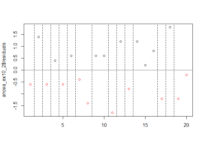
Runs Test와 Durbin-Watson test을 통하여 잔차의 자기상관성을 확인하여 보겠다.

Runs Test

anova_ex10_2 <- aov(ex10_2$exam10_2.phosphorus~as.factor(ex10_2$exam10_2.technician))
runs.test(anova_ex10_2$residuals, alternative = "two.sided", threshold = 0, plot = TRUE)

## 
##  Runs Test - Two sided
## 
## data:  anova_ex10_2$residuals
## Standardized Runs Statistic = 1.8379, p-value = 0.06608

p-value = 0.06608로써 만족스럽게 귀무가설을 기각하지 못하였다.

Durbin-Watson test

dwtest(anova_ex10_2, alternative = "greater")

## 
##  Durbin-Watson test
## 
## data:  anova_ex10_2
## DW = 3.228, p-value = 0.994
## alternative hypothesis: true autocorrelation is greater than 0

Durbin-Watson test의 경우 DW = 3.228로써 4에 가까운 값이 나왔으며, 2보다 크므로 alternative = “greater” 주었고 p-value = 0.994로 귀무가설 “자기상관이 0 이다.”를 기각하지 못한다.
자기상관성이 없다고 독립인 건 아니지만 독립성 가정이 만족된다고 가정할 수 있을 것 같다.
표본이 정규분포를 따르지 않지만 유사한 분포를 가지고 있고 분산도 유사하다면 Kruskal-Wallis Test가 적절하다.

kruskal.test(ex10_2$exam10_2.phosphorus~as.factor(ex10_2$exam10_2.technician))

## 
##  Kruskal-Wallis rank sum test
## 
## data:  ex10_2$exam10_2.phosphorus by as.factor(ex10_2$exam10_2.technician)
## Kruskal-Wallis chi-squared = 6.0065, df = 3, p-value = 0.1113

Kruskal-Wallis Test 결과 p-value가 0.1113으로 유의수준 0.05 보다 크기 때문에 귀무가설을 기각할 수 없고 따라서 유의수준 5%하에 인 함량의 모평균이 기술자마다 다르다고 말할만한 충분한 근거가 없다고 말할 수 있다.

EXAMPLE 10.3

#데이터셋
ex10_3

##    exam10_3.id exam10_3.variety exam10_3.potassium
## 1            1                1               27.9
## 2            2                1               27.0
## 3            3                1               26.0
## 4            4                1               26.5
## 5            5                1               27.0
## 6            6                1               27.5
## 7            7                2               24.2
## 8            8                2               24.7
## 9            9                2               25.6
## 10          10                2               26.0
## 11          11                2               27.4
## 12          12                2               26.1
## 13          13                3               29.1
## 14          14                3               27.7
## 15          15                3               29.9
## 16          16                3               30.7
## 17          17                3               28.8
## 18          18                3               31.1

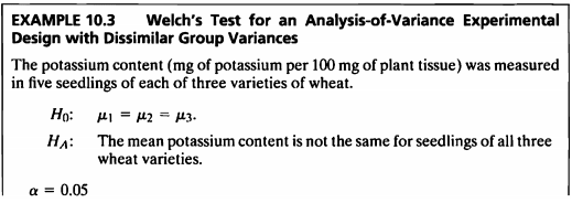
포타슘 함량(식물 조직 100mg당 포타슘의 mg)은 세 가지 종류의 밀 각각 6개의 모종에서 측정되었다.
본 검정의 가설은 다음과 같다.

\[\begin{aligned} H_0&:\ \mu_1=\mu_2=\mu_3\\ H_A&:\ The\ mean\ potassium\ content\ is\ not\ the\ same\ for\ seedlings\ of\ all\ three\ wheat\ varieties.\\ \end{aligned}\] \[\begin{aligned} F'&=\frac{\sum_{i=1}^k\ c_i(\bar{X}_i-\bar{X}_w)^2}{(k-1)[1+\frac{2A(k-2)}{K^2-1}]}\\\\ c_i&=\frac{n_i}{s_i^2},\ \ \ \ \ C=\sum_{i=1}^kc_i,\ \ \ \ \ \bar{X_w}=\frac{\sum_{i=1}^kc_i\bar{X_i}}{C},\ \ \ A=\sum_{i=1}^k\frac{(1-\frac{c_i}{C})^2}{v_i},\ where\ v_i=n_i-1 \\ For & \ critical \ value \ of \ F: \ v_1=k-1, \ v_2=\frac{k^2-1}{3A} \end{aligned}\]

Shapiro-Wilk Test로 네 그룹의 정규성을 평가하였다.

shapiro.test(subset(ex10_3$exam10_3.potassium,ex10_3$exam10_3.variety==1));shapiro.test(subset(ex10_3$exam10_3.potassium,ex10_3$exam10_3.variety==2));shapiro.test(subset(ex10_3$exam10_3.potassium,ex10_3$exam10_3.variety==3))

## 
##  Shapiro-Wilk normality test
## 
## data:  subset(ex10_3$exam10_3.potassium, ex10_3$exam10_3.variety == 1)
## W = 0.9778, p-value = 0.9401

## 
##  Shapiro-Wilk normality test
## 
## data:  subset(ex10_3$exam10_3.potassium, ex10_3$exam10_3.variety == 2)
## W = 0.96651, p-value = 0.8682

## 
##  Shapiro-Wilk normality test
## 
## data:  subset(ex10_3$exam10_3.potassium, ex10_3$exam10_3.variety == 3)
## W = 0.96881, p-value = 0.8844

Shapiro-Wilk test 결과 p-value가 0.05보다 매우 크므로 세 그룹 모두 모집단이 정규성을 따르지 않는다는 대립가설을 채택할 충분한 근거가 없다.
따라서 정규성을 만족한다는 사실을 바탕으로 그룹별 등분산성 검정을 진행한다.

class(ex10_3$exam10_3.variety)

## [1] "numeric"

variety의 class가 numeric이므로 factor로 변경해서 등분산성 검정을 실시한다.

Bartlett’s Test를 통해 네 그룹의 등분산성 검정을 진행하였다.

bartlett.test(ex10_3$exam10_3.potassium~as.factor(ex10_3$exam10_3.variety))

## 
##  Bartlett test of homogeneity of variances
## 
## data:  ex10_3$exam10_3.potassium by as.factor(ex10_3$exam10_3.variety)
## Bartlett's K-squared = 1.7512, df = 2, p-value = 0.4166

Bartlett’s Test의 유의확률은 p-value = 0.4166으로 유의수준 0.05보다 매우 크므로 등분산성이 아니라는 대립가설을 채택할 근거가 없다.
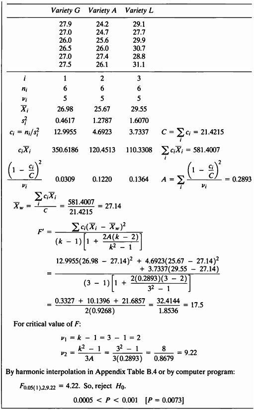
Runs Test와 Durbin-Watson test을 통하여 잔차의 자기상관성을 확인하여 보겠다.

Runs Test

anova_ex10_3 <- aov(ex10_3$exam10_3.potassium~as.factor(ex10_3$exam10_3.variety))
runs.test(anova_ex10_3$residuals, alternative = "two.sided", threshold = 0, plot = TRUE)

## 
##  Runs Test - Two sided
## 
## data:  anova_ex10_3$residuals
## Standardized Runs Statistic = -0.48591, p-value = 0.627

Runs Test 결과 p-value = 0.6616이므로 귀무가설 “연속적인 관측값이 임의적이다.”를 기각하지 못한다.

Durbin-Watson test

dwtest(anova_ex10_3, alternative = "less")

## 
##  Durbin-Watson test
## 
## data:  anova_ex10_3
## DW = 1.7019, p-value = 0.8811
## alternative hypothesis: true autocorrelation is less than 0

Durbin-Watson test의 경우 DW = 1.7019로써 0보다 2와 가깝게 나왔으며, 2보다 작으므로 alternative = “less” 주었고 p-value = 0.8811로 귀무가설 “자기상관이 0 이다.”를 기각하지 못한다.
자기상관성이 없다고 독립인 건 아니지만 독립성 가정이 만족된다고 가정할 수 있을 것 같다.
Shapiro-Wilk test와 Bartlett’s Test으로 정규성과 등분산성을 확인하였으므로 ANOVA 검정을 진행한다.

summary(aov(ex10_3$exam10_3.potassium~as.factor(ex10_3$exam10_3.variety)))

##                                    Df Sum Sq Mean Sq F value   Pr(>F)    
## as.factor(ex10_3$exam10_3.variety)  2  46.80  23.402   20.97 4.52e-05 ***
## Residuals                          15  16.74   1.116                     
## ---
## Signif. codes:  0 '***' 0.001 '**' 0.01 '*' 0.05 '.' 0.1 ' ' 1

p-value가 0.0000452으로 유의수준 0.05보다 매우 작기 때문에 귀무가설을 기각할 수 있고 따라서 유의수준 5%하에 그룹에 따라 밀의 칼륨 함유량의 모평균이 다르다고 말할 수 있다.
이 문제의 데이터는 정규성 가정과 등분산 가정을 만족하여 일원분산분석을 시행할 수 있지만, 문제에 나와 있는 대로 Welch’s test를 수행하도록 하겠다.
Welch’s test란 표본의 정규성은 만족되지만 그룹별 분산이 동일하지 않은 경우에 매우 강력한 검정이다.

Welch’s test

library(onewaytests)
welch.test(ex10_3$exam10_3.potassium~as.factor(ex10_3$exam10_3.variety),data=ex10_3)

## 
##   Welch's Heteroscedastic F Test (alpha = 0.05) 
## ------------------------------------------------------------- 
##   data : ex10_3$exam10_3.potassium and as.factor(ex10_3$exam10_3.variety) 
## 
##   statistic  : 15.0096 
##   num df     : 2 
##   denom df   : 9.218254 
##   p.value    : 0.00126072 
## 
##   Result     : Difference is statistically significant. 
## -------------------------------------------------------------

onewqy.test()에서 var.equal=F를 주면 같은 결과를 출력하여 준다.

oneway.test(ex10_3$exam10_3.potassium~as.factor(ex10_3$exam10_3.variety),var.equal=F)

## 
##  One-way analysis of means (not assuming equal variances)
## 
## data:  ex10_3$exam10_3.potassium and as.factor(ex10_3$exam10_3.variety)
## F = 15.01, num df = 2.0000, denom df = 9.2183, p-value = 0.001261

Welch’s test 결과도 동일하게 p-value가 유의수준 0.05보다 매우 작기 때문에 귀무가설을 기각할 수 있고 따라서 유의수준 5%하에 그룹에 따라 밀의 칼륨 함유량의 모평균이 다르다고 말할 수 있다.

EXAMPLE 10.4

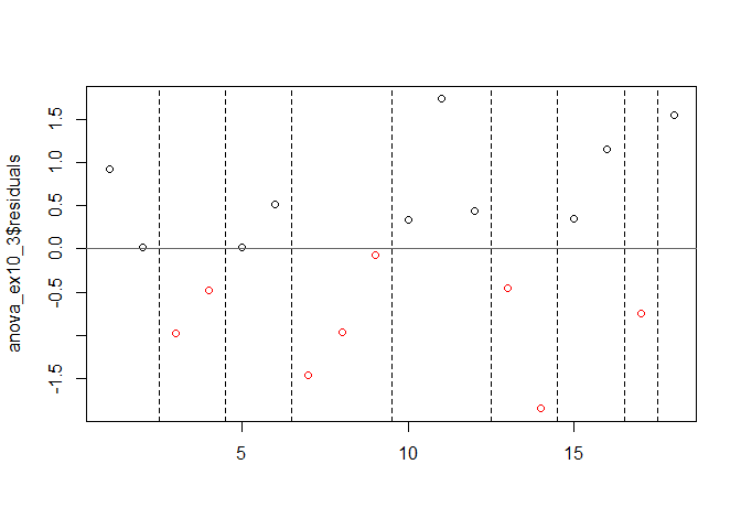
식물 뿌리 신장의 분산에 대한 제안된 분석은 4가지 화학 처리 각각에서 10개의 뿌리를 포함하는 것이다.
실험을 수행하고 실험에서 데이터를 수집하기 전에 제안된 시험의 검정력을 추정하는 것이 적절하고 바람직하다.
검정력을 계산할 때 대립가설 하에서 계산을 하게된다.
그 때 나오는 검정통계량은 \(\phi\) 를 따르게 되며 이를 구하는 공식및 결과는 다음과 같다.

\[\begin{aligned} \phi&=\sqrt{\frac{n\sum{(\mu_i-\mu)^2}}{ks^2}} \\ \mu&=\frac{\sum_{i=1}^k{\mu_i}}{k} \end{aligned}\]

문제에서 주어진 조건 하에서의 검정력을 구해 보자.

\[\begin{aligned} k&=4,\ \ \ \ \ \ \ \ \ n=10,\ \ \ \ \ \ \ \nu_1=k-1=3,\ \ \ \ \ \ \ \nu_2=k(n-1)=4(9)=36,\ \ \ \ \ \ \ \mu=\frac{8.0+8.0+9.0+12.0}{4}=9.25\\\\ \phi&=\sqrt{\frac{n\sum{(\mu_i-\mu)^2}}{ks^2}}=1.88 \end{aligned}\]

groups<-c(8,8,9,12)
power.anova.test(groups=4, n=10, between.var =var(groups), within.var = 7.5888, sig.level = 0.05, power=NULL)

## 
##      Balanced one-way analysis of variance power calculation 
## 
##          groups = 4
##               n = 10
##     between.var = 3.583333
##      within.var = 7.5888
##       sig.level = 0.05
##           power = 0.8621031
## 
## NOTE: n is number in each group

power=0.862로 높게 나왔다.
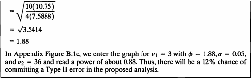
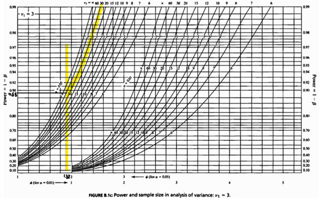
모집단 평균 간의 변동성이 지정된 경우 분산 분석의 검정력을 구할 수 있는 공식에 따라 \(\phi=1.88\) 나온다.
이를 이용해 power and sample size in analysis of variance: ν1=3 그래프에서 \(\phi=1.88\) 일때를 보면 그때의 검정력은 대략 0.88이고 이는 대립가설 하에서 제2종 오류를 범할 확률이 12%임을 의미한다.

EXAMPLE 10.5

최소 검출차가 주어졌을 때 분산의 검정력을 구하는 문제로써 구하는 공식은 다음과 같다.

\[\begin{aligned} \phi&=\sqrt{\frac{n\delta^2}{2ks^2}} \end{aligned}\]

공식을 함수로 작성하였다.

sample_size <- function(d,k,s,n){
  phi=sqrt((n*d^2)/(2*k*s))
  sample=data.frame(phi)
  return(sample)
}

문제에서 주어진 조건하에 공식에 대입하여 보자.

\[\begin{aligned} k&=4,\ \ \ \ \ \ \ \ \ n=10,\ \ \ \ \ \ \ \nu_1=3,\ \ \ \ \ \ \ \nu_2=36,\ \ \ \ \ \delta=4.0mm,\ \ \ \ \ \ s^2=7.5888mm^2\\\\ \phi&=\sqrt{\frac{n\delta^2}{2ks^2}}=1.62 \end{aligned}\]

작성한 sample_size 공식에 대입하여 \(\phi\)를 구하였다.

sample_size(d=4, k=4, s=7.5888, n=10)%>%
  kbl(caption = "Result") %>%
  kable_styling(bootstrap_options = c("striped", "hover", "condensed", "responsive"))

Result
phi
1.623411

다음은 pwr.1way 함수를 이용하여 power을 구하였다.

library(pwr2)
n <- 10
k <- 4
s2 <- 7.5888
delta<-4.0
phi<-round(sqrt((n*delta^2)/(2*k*s2)),2)
pwr.1way(k=4, n=10,f=NULL, alpha = 0.05, delta=4.0, sigma=sqrt(7.5888))

## 
##      Balanced one-way analysis of variance power calculation 
## 
##               k = 4
##               n = 10
##           delta = 4
##           sigma = 2.754778
##     effect.size = 0.5133676
##       sig.level = 0.05
##           power = 0.7348545
## 
## NOTE: n is number in each group, total sample = 40 power = 0.734854517715498

power=0.735로 나왔다.
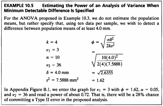
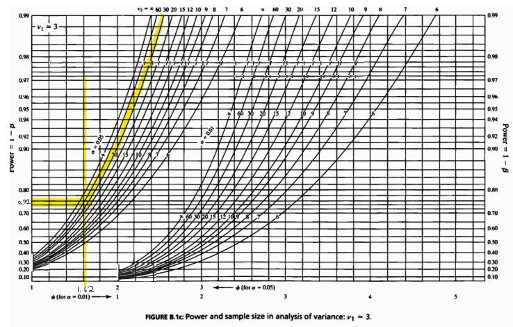
최소 검출 차가 지정된 경우 분산 분석의 검정력을 구할 수 있는 공식에 따라 \(\phi=1.62\)가 나온다
이를 이용해 power and sample size in analysis of variance: ν1=3 그래프에서 \(\phi=1.62\)일때를 보면 그때의 검정력은 대략 0.72이고 이는 대립가설 하에서 제2종 오류를 범할 확률이 28%임을 의미한다.
최소 탐지 가능한 차이가 지정된 경우 anova test의 power를 테스트하는 Balanced one-way analysis of variance power calculation 방법을 이용해 검정력을 구한 결과 또한 power=0.73으로 직접 구한 수치와 매우 유사한것을 볼 수 있다.

• 그룹 평균 간의 차이가 클수록 검정력은 커진다.

• 검정력은 표본 크기가 클수록 크다.

• 검정력은 더 적은 수의 그룹이 더 크다.

• 군내 변동성이 작을 경우 검정력이 더 크다.

• 검정력은 유의수준이 클수록 크다.

EXAMPLE 10.6

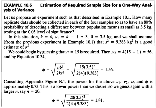
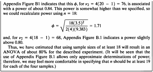
One-Way Analysis of Variance 에서 필요한 샘플사이즈를 구해보도록 한다.
80%의 확률로 3.5kg 만큼의 차이를 탐지하기 위해 필요한 샘플사이즈를 계산하여 보겠다.

\[\begin{aligned} k&=4,\ \ \ \ \ \ \ \ \ \nu_1=3,\ \ \ \ \ \ \ \ \delta=3.5kg,\ \ \ \ \ \ s^2=9.383kg^2\\\\ \phi&=\sqrt{\frac{n\delta^2}{2ks^2}} \end{aligned}\]

각 그룹에 대해 15만큼의 샘플이 필요하다고 가정하자

sample_size(d=3.5, k=4, s=9.383, n=15)%>%
  kbl(caption = "Result") %>%
  kable_styling(bootstrap_options = c("striped", "hover", "condensed", "responsive"))

Result
phi
1.56458

각 그룹에 대해 15만큼의 샘플이 필요하다고 가정하면 \(\phi=1.5645\)이고 표에서 찾아보면 이는 73%의 검정력에 해당한다.

각 그룹에 대해 20만큼의 샘플이 필요하다고 가정하자

sample_size(d=3.5, k=4, s=9.383, n=20)%>%
  kbl(caption = "Result") %>%
  kable_styling(bootstrap_options = c("striped", "hover", "condensed", "responsive"))

Result
phi
1.806622

각 그룹에 대해 20만큼의 샘플이 필요하다고 가정하면 \(\phi=1.80622\)이고 표에서 찾아보면 이는 84%의 검정력에 해당한다.

각 그룹에 대해 18만큼의 샘플이 필요하다고 가정하자

sample_size(d=3.5, k=4, s=9.383, n=18)%>%
  kbl(caption = "Result") %>%
  kable_styling(bootstrap_options = c("striped", "hover", "condensed", "responsive"))

Result
phi
1.713912

각 그룹에 대해 18만큼의 샘플이 필요하다고 가정하면 \(\phi=1.713912\)이고 표에서 찾아보면 이는 80%의 검정력에 거의 일치한다.
따라서 80% 이상의 검정력을 갖기 위해 필요한 최소한의 그룹별 샘플 사이즈는 18이라고 볼 수 있다.

EXAMPLE 10.7

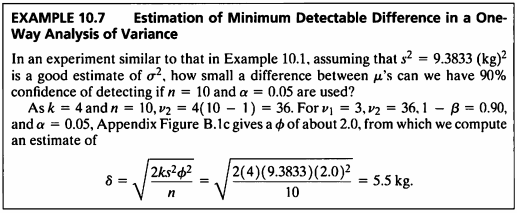
One-Way Analysis of Variance 에서 최소검출차를 구해보도록 한다.
ex10_1의 데이터를 이용하여 최소 검출차를 추정하기 위해 다음과 같은 공식을 이용하자.

\[\begin{aligned} \delta&=\sqrt{\frac{2ks^2\phi^2}{n}} \end{aligned}\]

주어진 대로 공식을 함수로 작성하였다.

Minimum_Detectable_Difference <- function(k,s,p,n){ 
  delta=sqrt((2*k*s*p^2)/n)
  mdd = data.frame(delta)
  return(mdd)
}

검정력: 90%, 그룹수: 4, 그룹별 샘플 수: 10, 유의수준: 0.05일 때 탐지할 수 있는 최소 검출차

Minimum_Detectable_Difference(k=4, s=9.3833, p=2.0, n=10)%>%
  kbl(caption = "Result") %>%
  kable_styling(bootstrap_options = c("striped", "hover", "condensed", "responsive"))

Result
delta
5.47965

검정력이 90%이고 그룹수는 4, 그룹별 샘플 수는 10, 유의수준은 0.05일 때 탐지할 수 있는 최소 검출차는 \(\delta=5.5\)로 계산되었다.
따라서 효과크기(최소검출차)=5.5일 때 집단간 차이가 유의하게 나타난다고 할 수 있다.

EXAMPLE 10.8

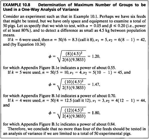
ex10_1과 같은 실험을 생각하여 볼 때 다음과 같은 가정을 하여보자.
6개의 사료를 테스트할 수 있지만, 총 50마리의 돼지를 검사할 수 있는 공간과 장비만 가지고 있다고 하자.
유의수준 0.05, 80이상의 검정력으로 테스트하고 모집단 평균 간의 4.5kg의 작은 차이를 발견하고자 한다.
One-Way Analysis of Variance에서 검정력과 유의수준이 정해져 있을 때 필요한 최대 그룹수를 구하도록 해본다.

\[\begin{aligned} \alpha&=0.05,\ \ \ \beta\leq0.20(power\ of\ at\ least\ 0.8),\ \ \ \ \delta=4.5\\ If\ k&=6,\ then\ n=\frac{50}{6}=8.3, \ \ \ \nu_1=5, \nu_2=6(8-1)=42 \end{aligned}\]

그룹 수 6으로 가정하자

sample_size(d=4.5, k=6, s=9.383, n=8)%>%
  kbl(caption = "Result") %>%
  kable_styling(bootstrap_options = c("striped", "hover", "condensed", "responsive"))

Result
phi
1.199488

그룹 수 6으로 가정하면 \(\phi=1.199488\)이다.

그룹 수 5로 가정하자

sample_size(d=4.5, k=5, s=9.383, n=10)%>%
  kbl(caption = "Result") %>%
  kable_styling(bootstrap_options = c("striped", "hover", "condensed", "responsive"))

Result
phi
1.469067

그룹 수 5로 가정하면 \(\phi=1.469067\)이다.

그룹 수 4로 가정하자

sample_size(d=4.5, k=4, s=9.383, n=12)%>%
  kbl(caption = "Result") %>%
  kable_styling(bootstrap_options = c("striped", "hover", "condensed", "responsive"))

Result
phi
1.799233

그룹 수 4로 가정하면 \(\phi=1.799233\)이다.
검정력이 80%일 때 \(\phi=1.8\)이므로 주어진 조건을 만족하기 위해서는 그룹 수를 4이하로 해야한다.
k=4라고 가정하고 power를 산출하여 보면 0.80이므로 그룹 수는 4개라고 할 수 있다.

EXAMPLE 10.9

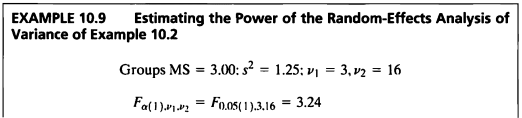
랜덤효과가 있는 분선분석의 검정력을 산출하는 공식은 다음과 같다.

\[\begin{aligned} Random-Effects\ of\ ANOVA&: \ F_{(1-\beta),\nu_1,\nu_2}=\frac{\nu_2s^2F_{\alpha(1),\nu_1,\nu_2}}{(\nu_2-2)(groups\ MS)} \end{aligned}\]

Example 10.2 데이터의 결과를 사용하여 ANOVA에서의 Random-Effect모델에서의 power를 구하여 보자.

\[\begin{aligned} Groups\ MS&=3.00,\ \ \ \ \ s^2=1.25,\ \ \ \ \ \nu_1=3,\ \ \ \ \nu_2=16\\\\ F_{\alpha(1),\nu_1,\nu_2}&=F_{0.05(1),3,16}=3.24\\\\ Random-Effects\ of\ ANOVA&: F_{(1-\beta),\nu_1,\nu_2}=\frac{\nu_2s^2F_{\alpha(1),\nu_1,\nu_2}}{(\nu_2-2)(groups\ MS)}=1.54 \end{aligned}\]

random_effect<-function(v1, v2, s, alpha, ms){
  F=((v2*s*qf(alpha, v1, v2, lower.tail = F))/((v2-2)*ms))
  f=data.frame(F)
  return(f)
}

계산 결과 F값은 1.54로 나왔으며, 이는 F분포표에서 자유도는 3과 16, 1-β 값이 0.1과 0.25 사이일 때 값임을 확인할 수 있다.
따라서 정확한 수치를 알수는 없지만 이들 사이의 값이 해당 분석의 검정력임을 알 수 있다.

random_effect(3, 16, 1.25, 0.05, 3.0)%>%
  kbl(caption = "Result") %>%
  kable_styling(bootstrap_options = c("striped", "hover", "condensed", "responsive"))

Result
F
1.54232

F_value <- random_effect(3, 16, 1.25, 0.05, 3.0)[1,]
pf(F_value, 3, 16, lower.tail = F)

## [1] 0.2421396

이 랜덤효과 모델의 검정력은 약 0.24임을 알 수 있다.

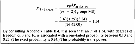
EXAMPLE 10.10

#데이터셋
ex10_10%>%
  kbl(caption = "Dataset",escape=F) %>%
  kable_styling(bootstrap_options = c("striped", "hover", "condensed", "responsive"))

Dataset
exam10_10.id	exam10_10.layer	exam10_10.abundance
1	1	14.0
2	1	12.1
3	1	9.6
4	1	8.2
5	1	10.2
6	2	8.4
7	2	5.1
8	2	5.5
9	2	6.6
10	2	6.3
11	3	6.9
12	3	7.3
13	3	5.8
14	3	4.1
15	3	5.4

한 곤충학자는 낙엽 활엽수림에서 파리 종의 수직 분포를 연구하고 있으며,
세 가지 다른 식물 층인 허브, 관목, 나무에서 각각 다섯 개의 파리 모음을 얻는다.
세 초목에 따른 파리들의 모이는 수의 분산에 차이가 있는지 검정해보도록 한다.

Shapiro-Wilk Test로 세 그룹의 정규성을 평가하였다.

shapiro.test(subset(ex10_10$exam10_10.abundance,ex10_10$exam10_10.layer==1));shapiro.test(subset(ex10_10$exam10_10.abundance,ex10_10$exam10_10.layer==2));shapiro.test(subset(ex10_10$exam10_10.abundance,ex10_10$exam10_10.layer==3))

## 
##  Shapiro-Wilk normality test
## 
## data:  subset(ex10_10$exam10_10.abundance, ex10_10$exam10_10.layer == 1)
## W = 0.97015, p-value = 0.8762

## 
##  Shapiro-Wilk normality test
## 
## data:  subset(ex10_10$exam10_10.abundance, ex10_10$exam10_10.layer == 2)
## W = 0.92329, p-value = 0.5514

## 
##  Shapiro-Wilk normality test
## 
## data:  subset(ex10_10$exam10_10.abundance, ex10_10$exam10_10.layer == 3)
## W = 0.95891, p-value = 0.8004

Shapiro-Wilk Test로 1,2,3 그룹 모두 정규성 검정한 결과 p-value가 0.05보다 매우 크므로 모집단이 정규성을 따르지 않는다는 대립가설을 채택할 충분한 근거가 없다.
등분산성 검정으로 Bartlett’s Test를 진행하여 보자.

class(ex10_10$exam10_10.layer)

## [1] "numeric"

layer의 class가 numeric이므로 factor로 변경해서 등분산성 검정을 실시한다.

Bartlett’s Test를 통해 네 그룹의 등분산성 검정을 진행하였다.

bartlett.test(ex10_10$exam10_10.abundance~as.factor(ex10_10$exam10_10.layer))

## 
##  Bartlett test of homogeneity of variances
## 
## data:  ex10_10$exam10_10.abundance by as.factor(ex10_10$exam10_10.layer)
## Bartlett's K-squared = 1.7057, df = 2, p-value = 0.4262

Bartlett’s Test의 유의확률은 p-value = 0.4262으로 유의수준 0.05보다 매우 크므로 등분산성이 아니라는 대립가설을 채택할 근거가 없다.
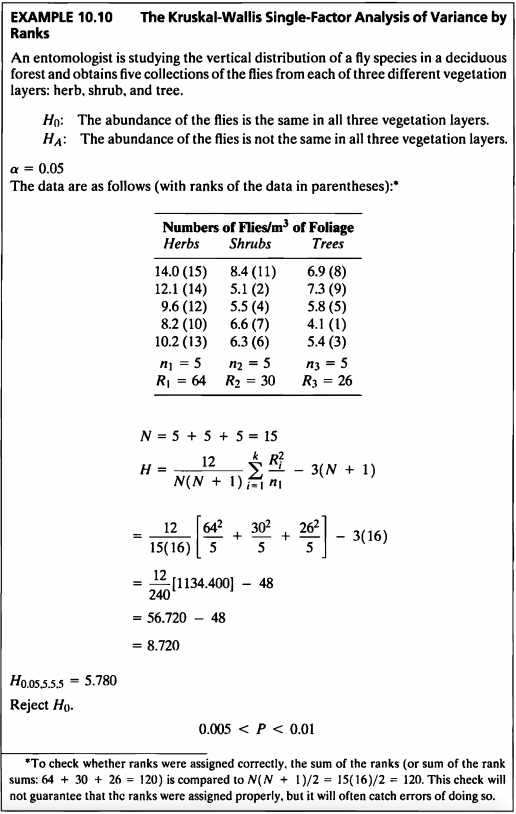
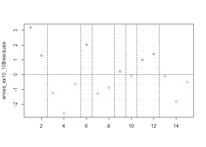
Runs Test와 Durbin-Watson test을 통하여 잔차의 자기상관성을 확인하여 보겠다.

Runs Test

anova_ex10_10 <- aov(ex10_10$exam10_10.abundance~as.factor(ex10_10$exam10_10.layer))
runs.test(anova_ex10_10$residuals, alternative = "two.sided", threshold = 0, plot = TRUE)

## 
##  Runs Test - Two sided
## 
## data:  anova_ex10_10$residuals
## Standardized Runs Statistic = -1.3282, p-value = 0.1841

p-value = 0.2658로써 귀무가설을 기각하지 못하였다.

Durbin-Watson test

dwtest(anova_ex10_10, alternative = "less")

## 
##  Durbin-Watson test
## 
## data:  anova_ex10_10
## DW = 1.2926, p-value = 0.9829
## alternative hypothesis: true autocorrelation is less than 0

Durbin-Watson test의 경우 DW = 1.2926로써 0보다 2와 가깝게 나왔으며, 2보다 작으므로 alternative = “less” 주었고 p-value = 0.9829로 귀무가설 “자기상관이 0 이다.”를 기각하지 못한다.
자기상관성이 없다고 독립인 건 아니지만 독립성 가정이 만족된다고 가정할 수 있을 것 같다.
정규성, 등분산성, 독립성이 만족되므로 ANOVA 검정을 실시한다.

summary(anova_ex10_10)

##                                    Df Sum Sq Mean Sq F value   Pr(>F)    
## as.factor(ex10_10$exam10_10.layer)  2  73.58   36.79   13.18 0.000937 ***
## Residuals                          12  33.50    2.79                     
## ---
## Signif. codes:  0 '***' 0.001 '**' 0.01 '*' 0.05 '.' 0.1 ' ' 1

p-value는 0.0009로 유의수준보다 매우 작기 때문에 귀무가설을 기각할 수 있고 따라서 식물에 따라 파리의 개체수 분포가 다르다고 말할 수 있다.
Kruskal-Wallis검정은 표본이 정규분포를 따르지 않지만 유사한 분포, 유사한 분산을 가질 때 적절한 비모수적 검정 방법이다.

kruskal.test(ex10_10$exam10_10.abundance~as.factor(ex10_10$exam10_10.layer))

## 
##  Kruskal-Wallis rank sum test
## 
## data:  ex10_10$exam10_10.abundance by as.factor(ex10_10$exam10_10.layer)
## Kruskal-Wallis chi-squared = 8.72, df = 2, p-value = 0.01278

같은 데이터에 대해 비모수적 방법, 즉 rank를 이용한 검정을 진행해 본 결과 p-value는 0.01278로써 유의수준보다 작기 때문에 귀무가설을 기각할 수 있다.
따라서 식물에 따라 파리의 개체수 분포가 다르다고 말할 수 있다.

library(pgirmess)
kruskalmc(ex10_10$exam10_10.abundance~as.factor(ex10_10$exam10_10.layer))

## Multiple comparison test after Kruskal-Wallis 
## p.value: 0.05 
## Comparisons
##     obs.dif critical.dif difference
## 1-2     6.8     6.771197       TRUE
## 1-3     7.6     6.771197       TRUE
## 2-3     0.8     6.771197      FALSE

Multiple comparison test after Kruskal-Wallis 실시한 결과 유의수준 5%하에 1-2, 1-3 그룹간 차이가 있다고 말할 수 있다.

EXAMPLE 10.11

#데이터셋
ex10_11%>%
  kbl(caption = "Dataset",escape=F) %>%
  kable_styling(bootstrap_options = c("striped", "hover", "condensed", "responsive"))

Dataset
exam10_11.id	exam10_11.pond	exam10_11.ph
1	1	7.68
2	1	7.69
3	1	7.70
4	1	7.70
5	1	7.72
6	1	7.73
7	1	7.73
8	1	7.76
9	2	7.71
10	2	7.73
11	2	7.74
12	2	7.74
13	2	7.78
14	2	7.78
15	2	7.80
16	2	7.81
17	3	7.74
18	3	7.75
19	3	7.77
20	3	7.78
21	3	7.80
22	3	7.81
23	3	7.84
24	4	7.71
25	4	7.71
26	4	7.74
27	4	7.79
28	4	7.81
29	4	7.85
30	4	7.87
31	4	7.91

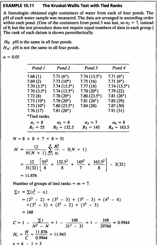
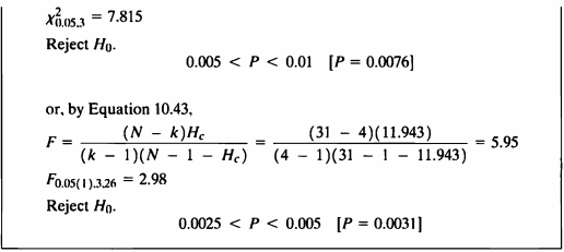
이 예제는 데이터 정렬 후 tied rank 데이터가 있는 비모수 anova 검정을 사용하는 예제이다.
데이터는 4개의 연못에서의 산성도를 측정한 데이터이다.
가설은 다음과 같다.

\[\begin{aligned} H_0&: pH\ is\ the\ same\ in\ all\ four\ ponds.\\ H_A&: pH\ is\ not\ the\ same\ in\ all\ four\ ponds.\\ \end{aligned}\]

네 연못의 pH농도가 같은지 검정하기 위해 먼저 그룹별 정규성 검정을 한다.

Shapiro-Wilk Test로 세 그룹의 정규성을 평가하였다.

shapiro.test(subset(ex10_11$exam10_11.ph,ex10_11$exam10_11.pond==1));shapiro.test(subset(ex10_11$exam10_11.ph,ex10_11$exam10_11.pond==2));shapiro.test(subset(ex10_11$exam10_11.ph,ex10_11$exam10_11.pond==3));shapiro.test(subset(ex10_11$exam10_11.ph,ex10_11$exam10_11.pond==4))

## 
##  Shapiro-Wilk normality test
## 
## data:  subset(ex10_11$exam10_11.ph, ex10_11$exam10_11.pond == 1)
## W = 0.95, p-value = 0.7113

## 
##  Shapiro-Wilk normality test
## 
## data:  subset(ex10_11$exam10_11.ph, ex10_11$exam10_11.pond == 2)
## W = 0.92959, p-value = 0.5123

## 
##  Shapiro-Wilk normality test
## 
## data:  subset(ex10_11$exam10_11.ph, ex10_11$exam10_11.pond == 3)
## W = 0.97382, p-value = 0.9245

## 
##  Shapiro-Wilk normality test
## 
## data:  subset(ex10_11$exam10_11.ph, ex10_11$exam10_11.pond == 4)
## W = 0.93368, p-value = 0.5502

Shapiro-Wilk Test로 1,2,3,4 그룹 모두 정규성 검정한 결과 p-value가 0.05보다 매우 크므로 모집단이 정규성을 따르지 않는다는 대립가설을 채택할 충분한 근거가 없다.
등분산성 검정으로 Bartlett’s Test를 진행하여 보자.

class(ex10_11$exam10_11.pond)

## [1] "numeric"

pond의 class가 numeric이므로 factor로 변경해서 등분산성 검정을 실시한다.

Bartlett’s Test를 통해 네 그룹의 등분산성 검정을 진행하였다.

bartlett.test(ex10_11$exam10_11.ph~as.factor(ex10_11$exam10_11.pond))

## 
##  Bartlett test of homogeneity of variances
## 
## data:  ex10_11$exam10_11.ph by as.factor(ex10_11$exam10_11.pond)
## Bartlett's K-squared = 8.8272, df = 3, p-value = 0.03168

Bartlett’s Test의 유의확률은 p-value = 0.03168으로 유의수준 0.05보다 작으므로 등분산성이 아니라는 대립가설을 채택할 근거가 있다.
따라서 이 예제는 등분산성 가정을 만족하지 못한다.
등분산성 가정이 위배된 경우의 ANOVA test로 Welch’s test와 Brown and Forsythe 방법을 사용한다.

Welch’s test는 그룹별 표본크기는 동일하나 모분산이 동일하지 않은 경우 더 우수하지만 데이터의 분포가 매우 치우친 분포인 경우 귀무가설을 쉽게 기각하는 단점이 있다.

Brown and Forsythe 방법은 극단적인 평균값이 큰 분산과 관련 있는 경우에 검정력이 더 크다.

이 예제의 경우 Kruskal-Wallis test로 진행하였으므로 Kruskal-Wallis test를 진행하여 보자.

등분산성이 만족되지 않고 그룹별 샘플 수가 다르므로 비모수적 방법인 Kruskal-Wallis test 진행하여보자.

kruskal.test(ex10_11$exam10_11.ph~as.factor(ex10_11$exam10_11.pond))

## 
##  Kruskal-Wallis rank sum test
## 
## data:  ex10_11$exam10_11.ph by as.factor(ex10_11$exam10_11.pond)
## Kruskal-Wallis chi-squared = 11.944, df = 3, p-value = 0.007579

p=0.0076로 귀무가설을 기각하므로 PH는 모든 네 개 연못이 같다고 할 수 없다.
Kruskal-Wallis test에서 처리간의 차이가 있다고 할 때, 추가적으로 어느 처리에서 차이가 있는지 확인하여보자.
R에서 pgirmess 패키지의 kruskalmc() 함수를 사용하여 순위합 개념을 이용한 다중비교 검정을 하겠다.

kruskalmc(ex10_11$exam10_11.ph, as.factor(ex10_11$exam10_11.pond))

## Multiple comparison test after Kruskal-Wallis 
## p.value: 0.05 
## Comparisons
##        obs.dif critical.dif difference
## 1-2  9.6875000     11.99368      FALSE
## 1-3 13.8392857     12.41464       TRUE
## 1-4 13.5625000     11.99368       TRUE
## 2-3  4.1517857     12.41464      FALSE
## 2-4  3.8750000     11.99368      FALSE
## 3-4  0.2767857     12.41464      FALSE

결과를 확인하여 보면, 유의수준 0.05하에서 1-3, 1-4 차이가 있다고 할 수 있다.
4 그룹의 분산을 각각 확인하여 보면,

var(ex10_11[ex10_11$exam10_11.pond==1,3]);var(ex10_11[ex10_11$exam10_11.pond==2,3]);var(ex10_11[ex10_11$exam10_11.pond==3,3]);var(ex10_11[ex10_11$exam10_11.pond==4,3])

## [1] 0.0006839286

## [1] 0.001298214

## [1] 0.001228571

## [1] 0.005641071

각 그룹별 분산의 크기가 매우 작은 것을 볼 수 있다.
등분산성 가정이 위배되고 낮은 분산을 취했으므로 Welch’s test 비모수적 검정을 통하여 네 연못의 모평균 pH가 같은지 여부를 검정하여 보겠다.

welch.test(ex10_11$exam10_11.ph~as.factor(ex10_11$exam10_11.pond),data=ex10_11)

## 
##   Welch's Heteroscedastic F Test (alpha = 0.05) 
## ------------------------------------------------------------- 
##   data : ex10_11$exam10_11.ph and as.factor(ex10_11$exam10_11.pond) 
## 
##   statistic  : 7.898356 
##   num df     : 3 
##   denom df   : 14.37493 
##   p.value    : 0.002369379 
## 
##   Result     : Difference is statistically significant. 
## -------------------------------------------------------------

p-value가 유의수준 0.05보다 작기 때문에 귀무가설을 기각할 수 있으며 연못에 따라 pH농도의 모평균 차이가 있다고 말할 수 있다.
등분산성이 만족되지 않고 그룹별 샘플 수가 다를 때 사용할 수 있는 사후검정법으로 Dunnett’s C test를 진행하여보겠다.
R에서 DescTools 패키지의 DunnettTest() 함수를 사용하겠다.

library(DescTools)
DunnettTest(ex10_11$exam10_11.ph~as.factor(ex10_11$exam10_11.pond),control=1);DunnettTest(ex10_11$exam10_11.ph~as.factor(ex10_11$exam10_11.pond),control=2);DunnettTest(ex10_11$exam10_11.ph~as.factor(ex10_11$exam10_11.pond),control=3)

## 
##   Dunnett's test for comparing several treatments with a control :  
##     95% family-wise confidence level
## 
## $`1`
##           diff       lwr.ci    upr.ci   pval    
## 2-1 0.04750000 -0.011567833 0.1065678 0.1360    
## 3-1 0.07053571  0.009394699 0.1316767 0.0211 *  
## 4-1 0.08500000  0.025932167 0.1440678 0.0037 ** 
## 
## ---
## Signif. codes:  0 '***' 0.001 '**' 0.01 '*' 0.05 '.' 0.1 ' ' 1

## 
##   Dunnett's test for comparing several treatments with a control :  
##     95% family-wise confidence level
## 
## $`2`
##            diff      lwr.ci     upr.ci   pval    
## 1-2 -0.04750000 -0.10656783 0.01156783 0.1359    
## 3-2  0.02303571 -0.03810530 0.08417673 0.6748    
## 4-2  0.03750000 -0.02156783 0.09656783 0.2866    
## 
## ---
## Signif. codes:  0 '***' 0.001 '**' 0.01 '*' 0.05 '.' 0.1 ' ' 1

## 
##   Dunnett's test for comparing several treatments with a control :  
##     95% family-wise confidence level
## 
## $`3`
##            diff      lwr.ci       upr.ci   pval    
## 1-3 -0.07053571 -0.13142822 -0.009643206 0.0203 *  
## 2-3 -0.02303571 -0.08392822  0.037856794 0.6644    
## 4-3  0.01446429 -0.04642822  0.075356794 0.8802    
## 
## ---
## Signif. codes:  0 '***' 0.001 '**' 0.01 '*' 0.05 '.' 0.1 ' ' 1

결과를 확인하여 보면 그룹 3과 그룹1, 그룹4와 그룹1의 p-value가 0.05보다 작게 나왔다.
따라서 연못1과 연못3, 그리고 연못1과 연못4의 모평균 pH농도가 다르다고 말할 수 있다.

EXAMPLE 10.12

#데이터셋
ex10_12%>%
  kbl(caption = "Dataset",escape=F) %>%
  kable_styling(bootstrap_options = c("striped", "hover", "condensed", "responsive"))

Dataset
exam10_12.id	exam10_12.side	exam10_12.height
1	1	7.1
2	1	7.2
3	1	7.4
4	1	7.6
5	1	7.6
6	1	7.7
7	1	7.7
8	1	7.9
9	1	8.1
10	1	8.4
11	1	8.5
12	1	8.8
13	2	6.9
14	2	7.0
15	2	7.1
16	2	7.2
17	2	7.3
18	2	7.3
19	2	7.4
20	2	7.6
21	2	7.8
22	2	8.1
23	2	8.3
24	2	8.5
25	3	7.8
26	3	7.9
27	3	8.1
28	3	8.3
29	3	8.3
30	3	8.4
31	3	8.4
32	3	8.4
33	3	8.6
34	3	8.9
35	3	9.2
36	3	9.4
37	4	6.4
38	4	6.6
39	4	6.7
40	4	7.1
41	4	7.6
42	4	7.8
43	4	8.2
44	4	8.4
45	4	8.6
46	4	8.7
47	4	8.8
48	4	8.9

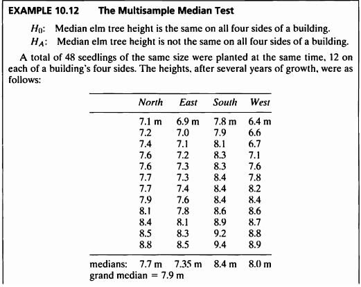
이 예제는 다표본 중위수 검정에 대한 예제이다.
데이터는 느릅나무의 길이를 건물의 4면에서 보았을 때의 높이를 기록한 데이터이다.
가설은 다음과 같다.

\[\begin{aligned} H_0&:Median\ elm\ tree\ height\ is\ the\ same\ on\ all\ four\ sides\ of\ a\ building.\\ H_A&:Median\ elm\ tree\ height\ is\ not\ the\ same\ on\ all\ four\ sides\ of\ a\ building.\\ &medians:7.7m\ \ \ 7.35m\ \ \ 8.4m \ \ \ 8.0m,\ \ \ grand\ median=7.9m\\ \end{aligned}\]

느릅나무 높이의 중앙값이 건물의 4면 모두에서 동일한지 검정하기 위해 먼저 각 샘플에 대해 정규성 검정을 진행한다.

Shapiro-Wilk Test로 세 그룹의 정규성을 평가하였다.

shapiro.test(subset(ex10_12$exam10_12.height,ex10_12$exam10_12.side==1));shapiro.test(subset(ex10_12$exam10_12.height,ex10_12$exam10_12.side==2));shapiro.test(subset(ex10_12$exam10_12.height,ex10_12$exam10_12.side==3));shapiro.test(subset(ex10_12$exam10_12.height,ex10_12$exam10_12.side==4))

## 
##  Shapiro-Wilk normality test
## 
## data:  subset(ex10_12$exam10_12.height, ex10_12$exam10_12.side == 1)
## W = 0.95381, p-value = 0.6932

## 
##  Shapiro-Wilk normality test
## 
## data:  subset(ex10_12$exam10_12.height, ex10_12$exam10_12.side == 2)
## W = 0.91943, p-value = 0.2812

## 
##  Shapiro-Wilk normality test
## 
## data:  subset(ex10_12$exam10_12.height, ex10_12$exam10_12.side == 3)
## W = 0.93364, p-value = 0.4203

## 
##  Shapiro-Wilk normality test
## 
## data:  subset(ex10_12$exam10_12.height, ex10_12$exam10_12.side == 4)
## W = 0.89877, p-value = 0.1529

Shapiro-Wilk Test로 1,2,3,4 그룹 모두 정규성 검정한 결과 p-value가 0.05보다 매우 크므로 모집단이 정규성을 따르지 않는다는 대립가설을 채택할 충분한 근거가 없다.
등분산성 검정으로 Bartlett’s Test를 진행하여 보자.

class(ex10_12$exam10_12.side)

## [1] "numeric"

side의 class가 numeric이므로 factor로 변경해서 등분산성 검정을 실시한다.

Bartlett’s Test를 통해 네 그룹의 등분산성 검정을 진행하였다.

bartlett.test(ex10_12$exam10_12.height~as.factor(ex10_12$exam10_12.side))

## 
##  Bartlett test of homogeneity of variances
## 
## data:  ex10_12$exam10_12.height by as.factor(ex10_12$exam10_12.side)
## Bartlett's K-squared = 6.4423, df = 3, p-value = 0.09196

Bartlett’s Test의 유의확률은 p-value = 0.09196으로 유의수준 0.05보다 크므로 등분산성이 아니라는 대립가설을 채택할 근거가 없다.
따라서 이 예제는 등분산성 가정을 만족한다.
중앙값에 대한 검정 중 비모수적인 방법인 Mood’s median test를 수행하도록 한다.
R에서 RVAideMemoire패키지의 mood.medtest() 함수를 사용하였다.

median=median(ex10_12$exam10_12.height)
ex10_12$height <- ex10_12$exam10_12.height # height의 중앙값을 NA로 만들어줄 변수 생성
ex10_12$height[ex10_12$exam10_12.height == median]<-NA # height의 중앙값을 NA로 변경
ex10_12_na_rm<-na.omit(ex10_12) # height의 중앙값 7.9 제거
mood.medtest(ex10_12_na_rm$height~ex10_12_na_rm$exam10_12.side, data=ex10_12_na_rm, exact=F)

## 
##  Mood's median test
## 
## data:  ex10_12_na_rm$height by ex10_12_na_rm$exam10_12.side
## X-squared = 11.182, df = 3, p-value = 0.01078

Mood’s median test 검정 결과 p-value=0.01078으로 유의수준 0.05하에 귀무가설을 기각할 충분한 근거가 있다.
따라서 건물 4면에 서 보는 방향에 따라 느릅나무의 길이에 대한 중앙값의 분포에 차이가 있다는 충분한 근거가 있다.

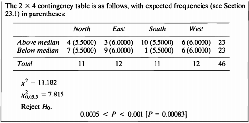
카이제곱 검정

해당 문제는 분할표자료에서 카이제곱 검정을 수행해도 된다.
검정과정
모든 관측치를 통합한 수 중위수를 구한다.
중위수보다 크거나 작은 관측치의 개수를 센다.
분할표를 작성한다.
카이제곱 검정을 한다.

	North	East	South	West
Above median	4(5.5)	3(6.0)	10(5.5)	6(6.0)	23
Not above median	7(5.5)	9(6.0)	1(5.5)	6(6.0)	23
Total	11	12	11	12	46

\[\begin{aligned} \chi^2=11.182,\ \ \ \chi_{0.05,3}^2=7.815\ \ \rightarrow Reject\ H_0.\\ 0.0005<P<0.001\ \ \ \ [P=0.00083] \end{aligned}\]

EXAMPLE 10.13

#데이터셋
ex10_13%>%
  kbl(caption = "Dataset",escape=F) %>%
  kable_styling(bootstrap_options = c("striped", "hover", "condensed", "responsive"))

Dataset
exam10_13.id	exam10_13.diet	exam10_13.weight
1	1	60.8
2	1	67.0
3	1	65.0
4	1	68.6
5	1	61.7
6	2	68.7
7	2	67.7
8	2	75.0
9	2	73.3
10	2	71.8
11	3	69.6
12	3	77.1
13	3	75.2
14	3	71.5
15	3	NA
16	4	61.9
17	4	64.2
18	4	63.1
19	4	66.7
20	4	60.3

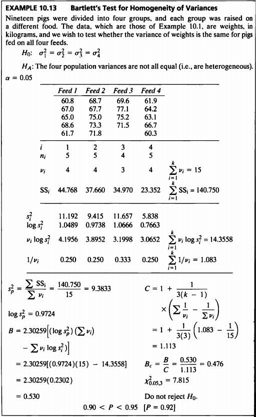
이 예제는 Example 10.1 데이터를 사용하여 분산의 동질성 검정을 하는 예제이다.

\[\begin{aligned} H_0&: \sigma_1^2=\sigma_2^2=\sigma_3^2=\sigma_4^2\\ H_A&: The\ four\ population\ variances\ are\ not\ all\ equal.\\ B&=(ln{s_p}^2)(\sum_{i=1}^k{\nu_i})-\sum_{i=1}^k\nu_i\ ln{s_i^2}=0.530\\\\ C&=1+\frac{1}{3(k-1)}(\sum_{i=1}^k{\frac{1}{\nu_i}-\frac{1}{\sum_{i=1}^k{\nu_i}}})=1.113\\ B_c&=\frac{B}{C}=0.476,\ \ \ \chi_{0.05,3}^2=7.815\ \ \ \ \ Do\ not\ reject\ H_0.\\ 0.9&<P<0.95\ \ \ \ [P=0.92] \end{aligned}\]

Example 10.1에서 보았듯이 네 그룹 모두 정규성 검정 결과 p-value가 0.05보다 매우 컸고 따라서 정규성을 만족하지 않는다고 볼만한 충분한 근거가 없었다.
정규성을 만족한다는 사실을 바탕으로 그룹별 등분산성 검정인 Bartlett’s Test를 진행한 결과 p-value가 0.9243으로 유의수준 0.05보다 매우 큰 수치이므로 귀무가설을 기각할 수 없고 따라서 네 그룹의 분산이 다르다고 볼만한 충분한 근거가 없다.

EXAMPLE 10-14

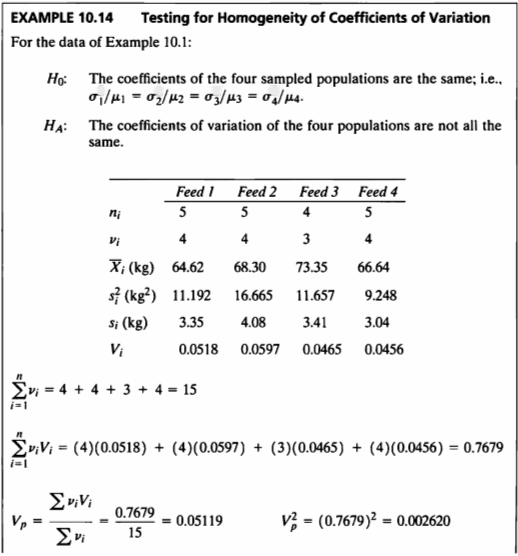
이 예제는 Example 10.1 데이터를 사용하여 변동계수에 대한 동질성 검정을 하는 예제이다.
본 검정의 가설은 다음과 같다.

\[\begin{aligned} H_0&: The\ coefficients\ of\ the\ four\ sampled\ populations\ are\ the\ same:\ i.e., \\ \\ &\frac{\sigma_1}{\mu_1}= \frac{\sigma_2}{\mu_2}= \frac{\sigma_3}{\mu_3}= \frac{\sigma_4}{\mu_4}\\ \\ H_A&: The\ coefficients\ of\ variation\ of\ the\ four\ populations\ are\ not\ all\ the\ same.\\ \end{aligned}\]

Homogeneity of Coefficients of variation 검정하는 함수를 작성하였다.

Homogeneity_CV<-function(n,m,ss){
  v<-n-1
  s<-sqrt(ss) 
  cv<-s/m
  vv=sum(v*cv)
  vp=sum(v*cv)/sum(v) 
  vp2=vp^2
  vv2=sum(v*(cv)^2)
  chisq=(vv2-(vv^2/sum(v)))/(vp2*(0.5+vp2)) 
  pvalue=pchisq(chisq,3, lower.tail=F) 
  return(data.frame(chisq,pvalue))
}

Homogeneity_CV(tapply(ex10_1$exam10_1.weight,as.factor(ex10_1$exam10_1.diet), length), tapply(ex10_1$exam10_1.weight,as.factor(ex10_1$exam10_1.diet), mean), tapply(ex10_1$exam10_1.weight,as.factor(ex10_1$exam10_1.diet), var))%>%
  kbl(caption = "Result") %>%
  kable_styling(bootstrap_options = c("striped", "hover", "condensed", "responsive"))

Result
chisq	pvalue
0.3873096	0.9428514

그룹 수가 여러 개일 때 변동계수의 동일성 검정을 위해 주어진 공식을 사용하여 검정통계량을 구한 결과 0.37이었고, 임계값은 7.815였다.
따라서 귀무가설을 기각할 수 없고 그룹별 변동계수가 같지 않다고 말할만한 충분한 근거가 없다.

SAS 프로그램 결과

SAS 접기/펼치기 버튼

10장

LIBNAME ex 'C:\Biostat';
RUN;

/*10장 연습문제 불러오기*/
%MACRO chap10(name=,no=);
%do i=1 %to &no.;
	PROC IMPORT DBMS=excel
		DATAFILE="C:\Biostat\data_chap10"
		OUT=ex.&name.&i. REPLACE;
		RANGE="exam10_&i.$";
	RUN;
%end;
%MEND;

%chap10(name=ex10_,no=13);

EXAMPLE 10.1

DATA exam_10_1;
    SET ex.ex10_1;
    if weight=. then delete;
RUN;

/*정규성 검정*/
ods graphics off;ods exclude all;ods noresults;
PROC UNIVARIATE DATA=ex.ex10_1 normal plot;
	CLASS diet;
	VAR weight;
	ods output TestsForNormality = TestsForNormality;
RUN;
ods graphics on;ods exclude none;ods results;
PROC SORT DATA=TestsForNormality;
	BY descending Test;
RUN;
title " ex10_1 : 정규성 가정";
PROC PRINT DATA=TestsForNormality label;
RUN;
title;

/*등분산성 검정*/
ods graphics off;ods exclude all;ods noresults;
PROC GLM DATA=ex.ex10_1;
	CLASS diet;
	MODEL weight=diet/p;
	MEANS diet / HOVTEST=BARTLETT;
	ods output Bartlett = Bartlett;
RUN;
ods graphics on;ods exclude none;ods results;


title "ex10_1 : 등분산 가정 (Bartlett's Test for Homogeneity of weight Variance)";
PROC PRINT DATA=Bartlett label;
RUN;
title;

/*독립성 검정*/
ods graphics off;ods exclude all;ods noresults;
PROC GLM DATA=ex.ex10_1;
	CLASS diet;
	MODEL weight=diet/p;
	output out=out_ds r=resid_var;
RUN;

DATA out_ds; 
	SET out_ds;
		time=_n_;
	ods graphics on;ods exclude none;ods results;
	PROC GPLOT DATA=out_ds;
		PLOT resid_var * time;
RUN;

/*anova*/
ods graphics off;ods exclude all;ods noresults;
PROC ANOVA data=ex.ex10_1;
	class diet;
	model weight=diet;
	means diet/ TUKEY hovtest=levene(type=abs);
    ods output OverallANOVA = OverallANOVA;
    ods output CLDiffs=CLDiffs;
run;
ods graphics on;ods exclude none;ods results;
PROC PRINT DATA=OverallANOVA; 
RUN;
PROC PRINT DATA=CLDiffs; 
RUN;

SAS 출력

ex10_1 : 정규성 가정


OBS	VarName	diet	적합도 검정	적합도 통계량에 대한 레이블	적합도 통계량 값	p-값 레이블	p-값의 부호	p-값
1	weight	1	Shapiro-Wilk	W	0.933155	Pr < W		0.6180
2	weight	2	Shapiro-Wilk	W	0.94389	Pr < W		0.6936
3	weight	3	Shapiro-Wilk	W	0.952018	Pr < W		0.7287
4	weight	4	Shapiro-Wilk	W	0.990268	Pr < W		0.9806
5	weight	1	Kolmogorov-Smirnov	D	0.208622	Pr > D	>	0.1500
6	weight	2	Kolmogorov-Smirnov	D	0.2016	Pr > D	>	0.1500
7	weight	3	Kolmogorov-Smirnov	D	0.206041	Pr > D	>	0.1500
8	weight	4	Kolmogorov-Smirnov	D	0.145566	Pr > D	>	0.1500
9	weight	1	Cramer-von Mises	W-Sq	0.035311	Pr > W-Sq	>	0.2500
10	weight	2	Cramer-von Mises	W-Sq	0.033613	Pr > W-Sq	>	0.2500
11	weight	3	Cramer-von Mises	W-Sq	0.034212	Pr > W-Sq	>	0.2500
12	weight	4	Cramer-von Mises	W-Sq	0.020098	Pr > W-Sq	>	0.2500
13	weight	1	Anderson-Darling	A-Sq	0.235734	Pr > A-Sq	>	0.2500
14	weight	2	Anderson-Darling	A-Sq	0.220699	Pr > A-Sq	>	0.2500
15	weight	3	Anderson-Darling	A-Sq	0.215876	Pr > A-Sq	>	0.2500
16	weight	4	Anderson-Darling	A-Sq	0.151062	Pr > A-Sq	>	0.2500

ex10_1 : 등분산 가정 (Bartlett's Test for Homogeneity of weight Variance)


OBS	Effect	Dependent	Source	DF	Chi-Square	Pr > ChiSq
1	diet	weight	diet	3	0.4752	0.9243


OBS	Dependent	Source	DF	SS	MS	FValue	ProbF
1	weight	Model	3	338.9373684	112.9791228	12.04	0.0003
2	weight	Error	15	140.7500000	9.3833333	_	_
3	weight	Corrected Total	18	479.6873684	_	_	_


OBS	Effect	Dependent	Method	Comparison	LowerCL	Difference	UpperCL	Significance
1	diet	weight	Tukey	3 - 2	-3.872	2.050	7.972	0
2	diet	weight	Tukey	3 - 1	2.808	8.730	14.652	1
3	diet	weight	Tukey	3 - 4	4.188	10.110	16.032	1
4	diet	weight	Tukey	2 - 3	-7.972	-2.050	3.872	0
5	diet	weight	Tukey	2 - 1	1.096	6.680	12.264	1
6	diet	weight	Tukey	2 - 4	2.476	8.060	13.644	1
7	diet	weight	Tukey	1 - 3	-14.652	-8.730	-2.808	1
8	diet	weight	Tukey	1 - 2	-12.264	-6.680	-1.096	1
9	diet	weight	Tukey	1 - 4	-4.204	1.380	6.964	0
10	diet	weight	Tukey	4 - 3	-16.032	-10.110	-4.188	1
11	diet	weight	Tukey	4 - 2	-13.644	-8.060	-2.476	1
12	diet	weight	Tukey	4 - 1	-6.964	-1.380	4.204	0

PROC IML;
USE exam_10_1;
READ all;
CLOSE exam_10_1;

k= ncol(unique(diet));
N_total=nrow(id);
sum_group=repeat(0, k);
group_mean=repeat(0, k);
group_n=repeat(0, k);
%MACRO loc(group);
%do i=1 %to 4 %by 1;
feed&i. = loc( &group= &i);
sum_group[&i.] = sum(weight[feed&i.]);
group_mean[&i.] = mean(weight[feed&i.]);
group_n[&i.]=nrow(weight[feed&i.]);
%end;
%MEND;
%loc(diet);

*(a);
sum_total = sum(sum_group);
mean_total = round(sum_total/nrow(weight), 0.0001);
mean_vec = repeat(mean_total, N_total);
totalSS = round((weight-mean_vec)`*(weight-mean_vec), 0.0001);
totalDF= N_total-1;
groupSS_el = repeat(0,k);
%MACRO groupSS_el;
%do i=1 %to 4 %by 1;
groupSS_el[&i.] = round(group_n[&i.]*((group_mean[&i.]-mean_total)**2), 0.0001);
group_mean_vec&i. = repeat(group_mean[&i.], group_n[&i.])`;
%end;
%MEND;
%groupSS_el;
groupSS = sum(groupSS_el);
groupDF=k-1;
group_mean_vec=(group_mean_vec1 || group_mean_vec2 || group_mean_vec3 ||group_mean_vec4)`;
SSE = (weight-group_mean_vec)`*(weight-group_mean_vec);
within_DF =sum(group_n-repeat(1,k));


*(b);
group_SS_first_el=repeat(0,k);
%MACRO group_SS_first;
%do i=1 %to 4 %by 1;
group_SS_first_el[&i.] = (sum_group[&i.]**2)/group_n[&i.];
%end;
%MEND;
%group_SS_first;
group_SS_first = sum(group_SS_first_el);
sum_weight = sum(weight);
sum_weightSquare = weight`*weight;

totalDF =  N_total-1;
groupsDF=k-1;
errorDF=N_total-k;

C=(sum_weight**2)/N_total;
b_totalSS = round(sum_weightSquare - C, 0.0001);
b_groupSS = round(group_SS_first - C, 0.0001);
b_errorSS = b_totalSS - b_groupSS;

*(c);
groupsMS = round( b_groupSS / groupsDF, 0.0001);
errorMS = round(b_errorSS/errorDF, 0.0001);
F = round(groupsMS /errorMS, 0.01);
critical_value = round(quantile('F', 1-0.05, groupsDF, errorDF), 0.01);
p_value = round(1- cdf('F', F, groupsDF, errorDF), 0.00001);

create exam10_1a_result var {totalSS totalDF groupSS groupDF SSE within_DF};
append; 
close exam10_1a_result;

create exam10_1b_result var {b_totalSS b_groupSS b_errorSS};
append; 
close exam10_1b_result;

create exam10_1c_result var {groupsMS errorMS F critical_value p_value};
append; 
close exam10_1c_result;

title "Example 10.1";
PRINT group_n sum_group group_mean;
RUN;
QUIT;

SAS 출력

Example 10.1

group_n	sum_group	group_mean
5	323.1	64.62
5	356.5	71.3
4	293.4	73.35
5	316.2	63.24

EXAMPLE 10.1a

title "Example 10.1 (a)";
PROC PRINT DATA=exam10_1a_result; 
RUN;

SAS 출력

Example 10.1 (a)


OBS	TOTALSS	TOTALDF	GROUPSS	GROUPDF	SSE	WITHIN_DF
1	479.687	18	338.937	3	140.75	15

EXAMPLE 10.1b

title "Example 10.1 (b)";
PROC PRINT DATA=exam10_1b_result; 
RUN;

SAS 출력

Example 10.1 (b)


OBS	B_TOTALSS	B_GROUPSS	B_ERRORSS
1	479.687	338.937	140.75

EXAMPLE 10.1c

title "Example 10.1 (c)";

%MACRO loc(data, group, y_var);
%do i=1 %to 4 %by 1;
group&i. = loc( &group= &i);
sum_group[&i.] = sum(&y_var[group&i.]);
group_mean[&i.] = mean(&y_var[group&i.]);
group_n[&i.]=nrow(&y_var[group&i.]);
%end;
%MEND;

%MACRO group_SS_first;
%do i=1 %to 4 %by 1;
group_SS_first_el[&i.] = (sum_group[&i.]**2)/group_n[&i.];
%end;
%MEND;

%MACRO anova(data, group, y_var, SSdec, pvaluedec);
PROC IML;
USE &data;
READ all;
CLOSE &data;

k= ncol(unique(&group));
N=nrow(id);
sum_group=repeat(0, k);
group_mean=repeat(0, k);
group_n=repeat(0, k);
%loc(&data, &group, &y_var);
sum_&y_var. = sum(&y_var);
sumSquare_&y_var. = &y_var`*&y_var;
C = (sum_&y_var. **2)/N;
totalSS = round( sumSquare_&y_var. - C, 0.0001);

group_SS_first_el=repeat(0,k);
%group_SS_first;
group_SS_first = sum(group_SS_first_el);
groupsSS = group_SS_first - C;
errorSS = totalSS - groupsSS;

totalDF =  N-1;
groupsDF = k-1;
errorDF = N-k;

groupsMS = round( groupsSS  / groupsDF, &SSdec);
errorMS = round(errorSS/errorDF, &SSdec);
F = round(groupsMS /errorMS, 0.01);
critical_value = round(quantile('F', 1-0.05, groupsDF, errorDF), 0.01);
p_value = round(1- cdf('F', F, groupsDF, errorDF), &pvaluedec);

PRINT F critical_value p_value;

RUN;
QUIT;
%MEND;

%anova(exam_10_1, diet, weight, 0.0001, 0.00001);

SAS 출력

Example 10.1 (c)

F	critical_value	p_value
12.04	3.29	0.00028

EXAMPLE 10.2

/*정규성 검정*/
ods graphics off;ods exclude all;ods noresults;
PROC UNIVARIATE DATA=ex.ex10_2 normal plot;
	CLASS technician;
	VAR phosphorus;
	ods output TestsForNormality = TestsForNormality;
RUN;
ods graphics on;ods exclude none;ods results;
PROC SORT DATA=TestsForNormality;
	BY descending Test;
RUN;
title " ex10_2 : 정규성 가정";
PROC PRINT DATA=TestsForNormality label;
RUN;
title;

/*독립성 검정*/
ods graphics off;ods exclude all;ods noresults;
PROC GLM DATA=ex.ex10_2;
	CLASS technician;
	MODEL phosphorus=technician/p;
	output out=out_ds r=resid_var;
RUN;
DATA out_ds; 
	SET out_ds;
	time=_n_;
	ods graphics on;ods exclude none;ods results;
PROC GPLOT DATA=out_ds;
	PLOT resid_var * time;
RUN;

/*등분산성*/
ods graphics off;ods exclude all;ods noresults;
PROC GLM DATA=ex.ex10_2 plots=(DIAGNOSTICS RESIDUALS);
	CLASS technician;
	MODEL phosphorus=technician;
	MEANS technician / HOVTEST=LEVENE(type=abs) hovtest=bf;
	ods output HOVFTest = HOVFTest;
RUN;
ods graphics on;ods exclude none;ods results;

title "ex10_2 : 등분산 가정 (Levene's Test & Brown and Forsythe's Test )";
PROC PRINT DATA=HOVFTest label;
RUN;
title;

/*KruskalWallisTest*/
ods graphics off;ods exclude all;ods noresults;
PROC NPAR1WAY DATA=ex.ex10_2 wilcoxon;
	ods trace on;
	CLASS technician;
	VAR phosphorus;
	ods output KruskalWallisTest=KruskalWallisTest;
RUN;
ods graphics on;ods exclude none;ods results;
title "ex10_2 : KruskalWallisTest";
PROC PRINT DATA=KruskalWallisTest label; 
RUN;

/*혼합모형  anova*/
ods graphics off;ods exclude all;ods noresults;
PROC MIXED DATA=ex.ex10_2  COVTEST CL;
	CLASS technician ;
	MODEL phosphorus= ;
	RANDOM technician  ; 
	ods output CovParms=CovParms;
RUN; 
QUIT; 
ods graphics on;ods exclude none;ods results;
title "ex10_2 : Covariance Parameter Estimates";
PROC PRINT DATA=CovParms label;
RUN;
title;

SAS 출력

ex10_2 : 정규성 가정


OBS	VarName	technician	적합도 검정	적합도 통계량에 대한 레이블	적합도 통계량 값	p-값 레이블	p-값의 부호	p-값
1	phosphorus	1	Shapiro-Wilk	W	0.770908	Pr < W		0.0460
2	phosphorus	2	Shapiro-Wilk	W	0.770908	Pr < W		0.0460
3	phosphorus	3	Shapiro-Wilk	W	0.90202	Pr < W		0.4211
4	phosphorus	4	Shapiro-Wilk	W	0.90202	Pr < W		0.4211
5	phosphorus	1	Kolmogorov-Smirnov	D	0.348833	Pr > D		0.0441
6	phosphorus	2	Kolmogorov-Smirnov	D	0.348833	Pr > D		0.0441
7	phosphorus	3	Kolmogorov-Smirnov	D	0.221307	Pr > D	>	0.1500
8	phosphorus	4	Kolmogorov-Smirnov	D	0.221307	Pr > D	>	0.1500
9	phosphorus	1	Cramer-von Mises	W-Sq	0.10627	Pr > W-Sq		0.0707
10	phosphorus	2	Cramer-von Mises	W-Sq	0.10627	Pr > W-Sq		0.0707
11	phosphorus	3	Cramer-von Mises	W-Sq	0.042471	Pr > W-Sq	>	0.2500
12	phosphorus	4	Cramer-von Mises	W-Sq	0.042471	Pr > W-Sq	>	0.2500
13	phosphorus	1	Anderson-Darling	A-Sq	0.602789	Pr > A-Sq		0.0519
14	phosphorus	2	Anderson-Darling	A-Sq	0.602789	Pr > A-Sq		0.0519
15	phosphorus	3	Anderson-Darling	A-Sq	0.288595	Pr > A-Sq	>	0.2500
16	phosphorus	4	Anderson-Darling	A-Sq	0.288595	Pr > A-Sq	>	0.2500

ex10_2 : 등분산 가정 (Levene's Test & Brown and Forsythe's Test )


OBS	Effect	Dependent	Method	Source	DF	Sum of Squares	Mean Square	F Value	Pr > F
1	technician	phosphorus	LV	technician	3	0.5120	0.1707	0.68	0.5755
2	technician	phosphorus	LV	Error	16	4.0000	0.2500	_	_
3	technician	phosphorus	BF	technician	3	0.8000	0.2667	0.41	0.7478
4	technician	phosphorus	BF	Error	16	10.4000	0.6500	_	_

ex10_2 : KruskalWallisTest


OBS	Variable	Chi-Square	Degrees of Freedom	Pr > Chi-Square
1	phosphorus	6.0065	3	0.1113

ex10_2 : Covariance Parameter Estimates


OBS	Cov Parm	Estimate	Standard Error	Z Value	Pr > Z	Alpha	Lower	Upper
1	technician	0.3500	0.4978	0.70	0.2410	0.05	0.06931	384.71
2	Residual	1.2500	0.4419	2.83	0.0023	0.05	0.6934	2.8953

EXAMPLE 10.3

/*정규성 검정*/
ods graphics off;ods exclude all;ods noresults;
PROC UNIVARIATE DATA=ex.ex10_3 normal plot;
	CLASS variety;
	VAR potassium;
	ods output TestsForNormality = TestsForNormality;
RUN;
ods graphics on;ods exclude none;ods results;
PROC SORT DATA=TestsForNormality;
	BY descending Test;
RUN;
title " ex10_3 : 정규성 가정";
PROC PRINT DATA=TestsForNormality label;
RUN;
title;

/*welch's anova*/
ods graphics off;ods exclude all;ods noresults;
PROC ANOVA data=ex.ex10_3;
	CLASS variety;
	MODEL potassium=variety;
	MEANS variety/  HOVTEST=BARTLETT welch;
	ods output Bartlett = Bartlett;
	ods output welch=welch;
RUN;
ods graphics on;ods exclude none;ods results;

title "ex10_3 : 등분산 가정 (Bartlett's Test for Homogeneity of weight Variance)";
PROC PRINT DATA=Bartlett;
RUN;
title;

title "ex10_3 : Welch's test";
PROC PRINT DATA=welch; 
RUN;
title;

ods graphics off;ods exclude all;ods noresults;
PROC UNIVARIATE DATA=ex.ex10_3 ;
	CLASS variety;
	VAR potassium;
	ods output moments=moments;
RUN;
ods graphics on;ods exclude none;ods results;
PROC PRINT DATA=moments; 
RUN;

SAS 출력

ex10_3 : 정규성 가정


OBS	VarName	variety	적합도 검정	적합도 통계량에 대한 레이블	적합도 통계량 값	p-값 레이블	p-값의 부호	p-값
1	potassium	1	Shapiro-Wilk	W	0.977796	Pr < W		0.9401
2	potassium	2	Shapiro-Wilk	W	0.966512	Pr < W		0.8682
3	potassium	3	Shapiro-Wilk	W	0.968814	Pr < W		0.8844
4	potassium	1	Kolmogorov-Smirnov	D	0.176451	Pr > D	>	0.1500
5	potassium	2	Kolmogorov-Smirnov	D	0.184113	Pr > D	>	0.1500
6	potassium	3	Kolmogorov-Smirnov	D	0.151176	Pr > D	>	0.1500
7	potassium	1	Cramer-von Mises	W-Sq	0.028922	Pr > W-Sq	>	0.2500
8	potassium	2	Cramer-von Mises	W-Sq	0.032192	Pr > W-Sq	>	0.2500
9	potassium	3	Cramer-von Mises	W-Sq	0.023808	Pr > W-Sq	>	0.2500
10	potassium	1	Anderson-Darling	A-Sq	0.17631	Pr > A-Sq	>	0.2500
11	potassium	2	Anderson-Darling	A-Sq	0.205577	Pr > A-Sq	>	0.2500
12	potassium	3	Anderson-Darling	A-Sq	0.171315	Pr > A-Sq	>	0.2500

ex10_3 : 등분산 가정 (Bartlett's Test for Homogeneity of weight Variance)


OBS	Effect	Dependent	Source	DF	ChiSq	ProbChiSq
1	variety	potassium	variety	2	1.7512	0.4166

ex10_3 : Welch's test


OBS	Effect	Dependent	Source	DF	FValue	ProbF
1	variety	potassium	variety	2.0000	15.01	0.0013
2	variety	potassium	Error	9.2183	_	_


OBS	VarName	variety	Label1	cValue1	nValue1	Label2	cValue2	nValue2
1	potassium	1	N	6	6.000000	가중합	6	6.000000
2	potassium	1	평균	26.9833333	26.983333	관측값 합	161.9	161.900000
3	potassium	1	표준 편차	0.67946057	0.679461	분산	0.46166667	0.461667
4	potassium	1	왜도	-0.1487695	-0.148770	첨도	-0.4470539	-0.447054
5	potassium	1	제곱합	4370.91	4370.910000	수정 제곱합	2.30833333	2.308333
6	potassium	1	변동계수	2.518075	2.518075	평균의 표준 오차	0.27738862	0.277389
7	potassium	2	N	6	6.000000	가중합	6	6.000000
8	potassium	2	평균	25.6666667	25.666667	관측값 합	154	154.000000
9	potassium	2	표준 편차	1.13078144	1.130781	분산	1.27866667	1.278667
10	potassium	2	왜도	0.26299788	0.262998	첨도	-0.0099899	-0.009990
11	potassium	2	제곱합	3959.06	3959.060000	수정 제곱합	6.39333333	6.393333
12	potassium	2	변동계수	4.40564198	4.405642	평균의 표준 오차	0.46163959	0.461640
13	potassium	3	N	6	6.000000	가중합	6	6.000000
14	potassium	3	평균	29.55	29.550000	관측값 합	177.3	177.300000
15	potassium	3	표준 편차	1.26767504	1.267675	분산	1.607	1.607000
16	potassium	3	왜도	-0.2292905	-0.229290	첨도	-0.9353331	-0.935333
17	potassium	3	제곱합	5247.25	5247.250000	수정 제곱합	8.035	8.035000
18	potassium	3	변동계수	4.28993244	4.289932	평균의 표준 오차	0.51752617	0.517526

EXAMPLE 10.4

PROC POWER;
	onewayanova
	groupmeans=8.0 |8.0|9.0|12.0
	stddev=2.754778
	alpha=0.05
	npergroup=10
    power=. ;
RUN;

PROC IML;
k=4;
n=10;
v1 = k-1;
v2 = k*(n-1);
means_i = {8.0 8.0 9.0 12.0}`;
mu = mean(means_i);
sigma_2=7.5888;
phi = round(sqrt((n*((means_i - repeat(mu, 4))`*(means_i - repeat(mu, 4))))/(k*sigma_2)), 0.01);

PRINT phi v1 v2 ;
RUN;
QUIT;

SAS 출력

The POWER Procedure

Overall F Test for One-Way ANOVA


Fixed Scenario Elements
Method	Exact
Alpha	0.05
Group Means	8 8 9 12
Standard Deviation	2.754778
Sample Size per Group	10


Computed Power
Power
0.862

phi	v1	v2
1.88	3	36

EXAMPLE 10.5

PROC IML;
	reset nolong;
	k=4;d=4;s=7.5888;n=10;
	p=sqrt((n*d*d)/(2*k*s));
	print p;
RUN;
QUIT;

/*결과 p=1.5645802*/

SAS 출력


p
1.6234108

EXAMPLE 10.6

PROC IML;
	reset nolong;
	k=4;d=3.5;s=9.383;n=15;
	p=sqrt((n*d*d)/(2*k*s));
	PRINT p;
RUN;
QUIT;

PROC IML;
	reset nolong;
	k=4;d=3.5;s=9.383;n=20;
	p=sqrt((n*d*d)/(2*k*s));
	PRINT p;
RUN;
QUIT;

PROC IML;
	reset nolong;
	k=4;d=3.5;s=9.383;n=18;
	p=sqrt((n*d*d)/(2*k*s));
	print p;
RUN;
QUIT;

/*결과 p=1.7139117*/

SAS 출력


p
1.5645802


p
1.8066216


p
1.7139117

EXAMPLE 10.7

PROC IML;
	reset nolong;
	k=4;p=2;s=9.383;n=10;
	d=sqrt((2*k*s*(p*p))/n);
	print d;
RUN;
QUIT;

SAS 출력


d
5.479562

EXAMPLE 10.8

PROC IML;
	reset nolong;
	d=4.5;s=9.383;
	p=sqrt((8*d*d)/(2*6*s));/*k=6라 가정하고 시행*/
	print p;
RUN;
QUIT;

PROC IML;
	reset nolong;
	d=4.5;s=9.383;
	p=sqrt((10*d*d)/(2*5*s));/*k=5라 가정하고 시행*/
	print p;
RUN;
QUIT;

PROC IML;
	reset nolong;
	d=4.5;s=9.383;
	p=sqrt((12*d*d)/(2*4*s));/*k=4라 가정하고 시행*/
	print p;
RUN;
QUIT;

/*k=4일때 power=0.80임을 알수있음*/

SAS 출력


p
1.1994883


p
1.4690672


p
1.7992325

EXAMPLE 10.9

PROC IML;
	reset nolong;
	gr_ms=3;s=1.25;v1=3;v2=16;
	F1=finv(1-0.05, v1,v2);
   F2=(v2*s*F1)/((v2-2)*(gr_ms));
   p=1-probF(F2,v1,v2);
   print F1 F2 p;
RUN;
QUIT;

SAS 출력

F1	F2	p
3.2388715	1.5423198	0.2421396

EXAMPLE 10.10

/*정규성 검정*/
ods graphics off;ods exclude all;ods noresults;
PROC UNIVARIATE DATA=ex.ex10_10 normal plot;
	CLASS layer;
	VAR abundance;
	ods output TestsForNormality = TestsForNormality;
RUN;
ods graphics on;ods exclude none;ods results;
PROC SORT DATA=TestsForNormality;
	BY descending Test;
RUN;
title " ex10_10 : 정규성 가정";
PROC PRINT DATA=TestsForNormality label;
RUN;
title;

/*등분산성 검정*/
ods graphics off;ods exclude all;ods noresults;
PROC GLM DATA=ex.ex10_10;
	CLASS layer;
	MODEL abundance=layer/p;
	MEANS layer / HOVTEST=BARTLETT;
	ods output Bartlett = Bartlett;
RUN;
ods graphics on;ods exclude none;ods results;


title "ex10_10 : 등분산 가정 (Bartlett's Test for Homogeneity of weight Variance)";
PROC PRINT DATA=Bartlett label;
RUN;
title;

/*anova*/
ods graphics off;ods exclude all;ods noresults;
PROC ANOVA DATA=ex.ex10_10;
	CLASS layer;
	MODEL abundance = layer;
	MEANS layer/ TUKEY hovtest=levene(type=abs);
	ods output OverallANOVA = OverallANOVA;
RUN;
ods graphics on;ods exclude none;ods results;
PROC PRINT DATA=OverallANOVA; 
RUN;
QUIT;

/*Kruskal-Wallis Test*/
ods graphics off;ods exclude all;ods noresults;
PROC NPAR1WAY DATA=ex.ex10_10;
	CLASS layer;
	VAR abundance;
	ods output KruskalWallisTest=KruskalWallisTest;
RUN;
ods graphics on;ods exclude none;ods results;

title "ex10_10 : Kruskal-Wallis Test";
PROC PRINT DATA=KruskalWallisTest; 
RUN;
title;
QUIT;

SAS 출력

ex10_10 : 정규성 가정


OBS	VarName	layer	적합도 검정	적합도 통계량에 대한 레이블	적합도 통계량 값	p-값 레이블	p-값의 부호	p-값
1	abundance	1	Shapiro-Wilk	W	0.970154	Pr < W		0.8762
2	abundance	2	Shapiro-Wilk	W	0.923293	Pr < W		0.5514
3	abundance	3	Shapiro-Wilk	W	0.958909	Pr < W		0.8004
4	abundance	1	Kolmogorov-Smirnov	D	0.207939	Pr > D	>	0.1500
5	abundance	2	Kolmogorov-Smirnov	D	0.231739	Pr > D	>	0.1500
6	abundance	3	Kolmogorov-Smirnov	D	0.184327	Pr > D	>	0.1500
7	abundance	1	Cramer-von Mises	W-Sq	0.029496	Pr > W-Sq	>	0.2500
8	abundance	2	Cramer-von Mises	W-Sq	0.042843	Pr > W-Sq	>	0.2500
9	abundance	3	Cramer-von Mises	W-Sq	0.028686	Pr > W-Sq	>	0.2500
10	abundance	1	Anderson-Darling	A-Sq	0.189383	Pr > A-Sq	>	0.2500
11	abundance	2	Anderson-Darling	A-Sq	0.278219	Pr > A-Sq	>	0.2500
12	abundance	3	Anderson-Darling	A-Sq	0.200353	Pr > A-Sq	>	0.2500

ex10_10 : 등분산 가정 (Bartlett's Test for Homogeneity of weight Variance)


OBS	Effect	Dependent	Source	DF	Chi-Square	Pr > ChiSq
1	layer	abundance	layer	2	1.7057	0.4262


OBS	Dependent	Source	DF	SS	MS	FValue	ProbF
1	abundance	Model	2	73.5840000	36.7920000	13.18	0.0009
2	abundance	Error	12	33.4960000	2.7913333	_	_
3	abundance	Corrected Total	14	107.0800000	_	_	_

ex10_10 : Kruskal-Wallis Test


OBS	Variable	ChiSquare	DF	Prob
1	abundance	8.7200	2	0.0128

EXAMPLE 10.11

/*정규성 검정*/
ods graphics off;ods exclude all;ods noresults;
PROC UNIVARIATE DATA=ex.ex10_11 normal plot;
	CLASS pond;
	VAR ph;
	ods output TestsForNormality = TestsForNormality;
RUN;
ods graphics on;ods exclude none;ods results;
PROC SORT DATA=TestsForNormality;
	BY descending Test;
RUN;
title " ex10_11 : 정규성 가정";
PROC PRINT DATA=TestsForNormality label;
RUN;
title;

/*등분산성 검정*/
ods graphics off;ods exclude all;ods noresults;
PROC GLM DATA=ex.ex10_11;
	CLASS pond;
	MODEL ph=pond/p;
	MEANS pond / HOVTEST=BARTLETT;
	ods output Bartlett = Bartlett;
RUN;
ods graphics on;ods exclude none;ods results;

title "ex10_11 : 등분산 가정 (Bartlett's Test for Homogeneity of weight Variance)";
PROC PRINT DATA=Bartlett label;
RUN;
title;

/*Kruskal-WallisTest*/
ods graphics off;ods exclude all;ods noresults;
PROC NPAR1WAY DATA=ex.ex10_11;
	CLASS pond;
	VAR ph;
	ods output KruskalWallisTest=KruskalWallisTest;
RUN;
ods graphics on;ods exclude none;ods results;

title "ex10_11 : Kruskal-Wallis Test";
PROC PRINT DATA=KruskalWallisTest; 
RUN;
title;
QUIT;

/*welch's anova*/
ods graphics off;ods exclude all;ods noresults;
PROC ANOVA data=ex.ex10_11;
	CLASS pond;
	MODEL ph=pond ;
	MEANS pond/  welch;
	ods output welch=welch;
RUN;
ods graphics on;ods exclude none;ods results;

title "ex10_11 : Welch's test";
PROC PRINT DATA=welch; 
RUN;
title;

SAS 출력

ex10_11 : 정규성 가정


OBS	VarName	pond	적합도 검정	적합도 통계량에 대한 레이블	적합도 통계량 값	p-값 레이블	p-값의 부호	p-값
1	ph	1	Shapiro-Wilk	W	0.950005	Pr < W		0.7113
2	ph	2	Shapiro-Wilk	W	0.929589	Pr < W		0.5123
3	ph	3	Shapiro-Wilk	W	0.97382	Pr < W		0.9245
4	ph	4	Shapiro-Wilk	W	0.933682	Pr < W		0.5502
5	ph	1	Kolmogorov-Smirnov	D	0.200477	Pr > D	>	0.1500
6	ph	2	Kolmogorov-Smirnov	D	0.222329	Pr > D	>	0.1500
7	ph	3	Kolmogorov-Smirnov	D	0.121718	Pr > D	>	0.1500
8	ph	4	Kolmogorov-Smirnov	D	0.157956	Pr > D	>	0.1500
9	ph	1	Cramer-von Mises	W-Sq	0.040945	Pr > W-Sq	>	0.2500
10	ph	2	Cramer-von Mises	W-Sq	0.058881	Pr > W-Sq	>	0.2500
11	ph	3	Cramer-von Mises	W-Sq	0.019496	Pr > W-Sq	>	0.2500
12	ph	4	Cramer-von Mises	W-Sq	0.032219	Pr > W-Sq	>	0.2500
13	ph	1	Anderson-Darling	A-Sq	0.255774	Pr > A-Sq	>	0.2500
14	ph	2	Anderson-Darling	A-Sq	0.325171	Pr > A-Sq	>	0.2500
15	ph	3	Anderson-Darling	A-Sq	0.150672	Pr > A-Sq	>	0.2500
16	ph	4	Anderson-Darling	A-Sq	0.24035	Pr > A-Sq	>	0.2500

ex10_11 : 등분산 가정 (Bartlett's Test for Homogeneity of weight Variance)


OBS	Effect	Dependent	Source	DF	Chi-Square	Pr > ChiSq
1	pond	ph	pond	3	8.8272	0.0317

ex10_11 : Kruskal-Wallis Test


OBS	Variable	ChiSquare	DF	Prob
1	ph	11.9435	3	0.0076

ex10_11 : Welch's test


OBS	Effect	Dependent	Source	DF	FValue	ProbF
1	pond	ph	pond	3.0000	7.90	0.0024
2	pond	ph	Error	14.3749	_	_

EXAMPLE 10.12

/*정규성 검정*/
ods graphics off;ods exclude all;ods noresults;
PROC UNIVARIATE DATA=ex.ex10_12 normal plot;
	CLASS side;
	VAR height;
	ods output TestsForNormality = TestsForNormality;
RUN;
ods graphics on;ods exclude none;ods results;
PROC SORT DATA=TestsForNormality;
	BY descending Test;
RUN;
title " ex10_12 : 정규성 가정";
PROC PRINT DATA=TestsForNormality label;
RUN;
title;

/*등분산성 검정*/
ods graphics off;ods exclude all;ods noresults;
PROC GLM DATA=ex.ex10_12;
	CLASS side;
	MODEL height=side/p;
	MEANS side/ HOVTEST=BARTLETT;
	ods output Bartlett = Bartlett;
RUN;
ods graphics on;ods exclude none;ods results;

title "ex10_12 : 등분산 가정 (Bartlett's Test for Homogeneity of weight Variance)";
PROC PRINT DATA=Bartlett label;
RUN;
title;

PROC NPAR1WAY DATA=ex.ex10_12 median correct=no;
	CLASS side;
	VAR height;
RUN;

DATA e_1012;
INPUT median $ side $ ex_f;
CARDS;
above north 4
above east 3
above south 10 
above west 6
below north 7
below east 9
below south 1
below west 6
;
RUN;

PROC FREQ DATA=e_1012 order=data;
    WEIGHT ex_f;
    TABLES median * side / nopercent nocol norow chisq;
RUN;

SAS 출력

ex10_12 : 정규성 가정


OBS	VarName	side	적합도 검정	적합도 통계량에 대한 레이블	적합도 통계량 값	p-값 레이블	p-값의 부호	p-값
1	height	1	Shapiro-Wilk	W	0.953812	Pr < W		0.6932
2	height	2	Shapiro-Wilk	W	0.919429	Pr < W		0.2812
3	height	3	Shapiro-Wilk	W	0.933638	Pr < W		0.4203
4	height	4	Shapiro-Wilk	W	0.898768	Pr < W		0.1529
5	height	1	Kolmogorov-Smirnov	D	0.183335	Pr > D	>	0.1500
6	height	2	Kolmogorov-Smirnov	D	0.189739	Pr > D	>	0.1500
7	height	3	Kolmogorov-Smirnov	D	0.228172	Pr > D		0.0835
8	height	4	Kolmogorov-Smirnov	D	0.161488	Pr > D	>	0.1500
9	height	1	Cramer-von Mises	W-Sq	0.046571	Pr > W-Sq	>	0.2500
10	height	2	Cramer-von Mises	W-Sq	0.070453	Pr > W-Sq	>	0.2500
11	height	3	Cramer-von Mises	W-Sq	0.074538	Pr > W-Sq		0.2286
12	height	4	Cramer-von Mises	W-Sq	0.068918	Pr > W-Sq	>	0.2500
13	height	1	Anderson-Darling	A-Sq	0.26929	Pr > A-Sq	>	0.2500
14	height	2	Anderson-Darling	A-Sq	0.413744	Pr > A-Sq	>	0.2500
15	height	3	Anderson-Darling	A-Sq	0.399729	Pr > A-Sq	>	0.2500
16	height	4	Anderson-Darling	A-Sq	0.459638	Pr > A-Sq		0.2219

ex10_12 : 등분산 가정 (Bartlett's Test for Homogeneity of weight Variance)


OBS	Effect	Dependent	Source	DF	Chi-Square	Pr > ChiSq
1	side	height	side	3	6.4423	0.0920

The NPAR1WAY Procedure


Median Scores (Number of Points Above Median) for Variable height Classified by Variable side
side	N	Sum of Scores	Expected Under H0	Std Dev Under H0	Mean Score
Average scores were used for ties.
1	12	4.50	6.0	1.483957	0.3750
2	12	3.00	6.0	1.483957	0.2500
3	12	10.50	6.0	1.483957	0.8750
4	12	6.00	6.0	1.483957	0.5000


Median One-Way Analysis
Chi-Square	DF	Pr > ChiSq
10.7283	3	0.0133

FREQ 프로시저

빈도


테이블 median * side
median	side
median	north	east	south	west	합계
above	4	3	10	6	23
below	7	9	1	6	23
합계	11	12	11	12	46

median * side 테이블에 대한 통계량


통계량	자유도	값	Prob
카이제곱	3	11.1818	0.0108
우도비 카이제곱	3	12.5154	0.0058
Mantel-Haenszel 카이제곱	1	2.4508	0.1175
파이 계수		0.4930
우발성 계수		0.4422
크래머의 V		0.4930

표본 크기 = 46

EXAMPLE 10.13

ods graphics off;ods exclude all;ods noresults;
PROC ANOVA DATA=exam_10_1;
	CLASS diet;
	MODEL weight=diet;
	MEANS diet/  hovtest= bartlett;
	ods output Bartlett=Bartlett;
RUN;
ods graphics on;ods exclude none;ods results;
PROC PRINT DATA=Bartlett;
RUN;

SAS 출력


OBS	Effect	Dependent	Source	DF	ChiSq	ProbChiSq
1	diet	weight	diet	3	0.4752	0.9243

EXAMPLE 10.14

PROC IML;
n={5, 5, 4, 5};
v={4, 4, 3, 4};
v_a={0.0518, 0.0597, 0.0465, 0.0456};
sum_v=sum(v);
sum_vv=sum(v#v_a);
v_p=sum_vv/sum_v;
v_p2=(v_p)**2;
sum_vv2=sum((v#v_a)#v_a);
chi_stat=round((sum_vv2-(((sum_vv)**2)/sum_v))/(v_p2*(0.5+v_p2)), 0.001);
chi_crit=round(abs(quantile("chisq", 1-0.05, 3)), 0.001);
PRINT sum_v sum_vv v_p v_p2 sum_vv2 chi_stat chi_crit;
RUN;
QUIT;

SAS 출력

sum_v	sum_vv	v_p	v_p2	sum_vv2	chi_stat	chi_crit
15	0.7679	0.0511933	0.0026208	0.0397935	0.366	7.815

교재: Biostatistical Analysis (5th Edition) by Jerrold H. Zar

**이 글은 22학년도 1학기 의학통계방법론 과제 자료들을 정리한 글 입니다.**

exam10_12.id	exam10_12.side	exam10_12.height
1	1	7.1
2	1	7.2
3	1	7.4
4	1	7.6
5	1	7.6
6	1	7.7
7	1	7.7
8	1	7.9
9	1	8.1
10	1	8.4
11	1	8.5
12	1	8.8
13	2	6.9
14	2	7.0
15	2	7.1
16	2	7.2
17	2	7.3
18	2	7.3
19	2	7.4
20	2	7.6
21	2	7.8
22	2	8.1
23	2	8.3
24	2	8.5
25	3	7.8
26	3	7.9
27	3	8.1
28	3	8.3
29	3	8.3
30	3	8.4
31	3	8.4
32	3	8.4
33	3	8.6
34	3	8.9
35	3	9.2
36	3	9.4
37	4	6.4
38	4	6.6
39	4	6.7
40	4	7.1
41	4	7.6
42	4	7.8
43	4	8.2
44	4	8.4
45	4	8.6
46	4	8.7
47	4	8.8
48	4	8.9

exam10_12.id	exam10_12.side	exam10_12.height
1	1	7.1
2	1	7.2
3	1	7.4
4	1	7.6
5	1	7.6
6	1	7.7
7	1	7.7
8	1	7.9
9	1	8.1
10	1	8.4
11	1	8.5
12	1	8.8
13	2	6.9
14	2	7.0
15	2	7.1
16	2	7.2
17	2	7.3
18	2	7.3
19	2	7.4
20	2	7.6
21	2	7.8
22	2	8.1
23	2	8.3
24	2	8.5
25	3	7.8
26	3	7.9
27	3	8.1
28	3	8.3
29	3	8.3
30	3	8.4
31	3	8.4
32	3	8.4
33	3	8.6
34	3	8.9
35	3	9.2
36	3	9.4
37	4	6.4
38	4	6.6
39	4	6.7
40	4	7.1
41	4	7.6
42	4	7.8
43	4	8.2
44	4	8.4
45	4	8.6
46	4	8.7
47	4	8.8
48	4	8.9

Multisample Hypotheses and the Analysis of Variance

R 프로그램 결과

10장

EXAMPLE 10.1

EXAMPLE 10.1a

EXAMPLE 10.1b

EXAMPLE 10.1c

EXAMPLE 10.2

EXAMPLE 10.3

EXAMPLE 10.4

EXAMPLE 10.5

EXAMPLE 10.6

EXAMPLE 10.7

EXAMPLE 10.8

EXAMPLE 10.9

EXAMPLE 10.10

EXAMPLE 10.11

EXAMPLE 10.12

EXAMPLE 10.13

EXAMPLE 10-14

SAS 프로그램 결과

10장

EXAMPLE 10.1

EXAMPLE 10.1a

EXAMPLE 10.1b

EXAMPLE 10.1c

EXAMPLE 10.2

EXAMPLE 10.3

EXAMPLE 10.4

EXAMPLE 10.5

EXAMPLE 10.6

EXAMPLE 10.7

EXAMPLE 10.8

EXAMPLE 10.9

EXAMPLE 10.10

EXAMPLE 10.11

EXAMPLE 10.12

EXAMPLE 10.13

EXAMPLE 10.14

Templates (for web app):

Error

Multisample Hypotheses and
the Analysis of Variance

exam10_12.id	exam10_12.side	exam10_12.height
1	1	7.1
2	1	7.2
3	1	7.4
4	1	7.6
5	1	7.6
6	1	7.7
7	1	7.7
8	1	7.9
9	1	8.1
10	1	8.4
11	1	8.5
12	1	8.8
13	2	6.9
14	2	7.0
15	2	7.1
16	2	7.2
17	2	7.3
18	2	7.3
19	2	7.4
20	2	7.6
21	2	7.8
22	2	8.1
23	2	8.3
24	2	8.5
25	3	7.8
26	3	7.9
27	3	8.1
28	3	8.3
29	3	8.3
30	3	8.4
31	3	8.4
32	3	8.4
33	3	8.6
34	3	8.9
35	3	9.2
36	3	9.4
37	4	6.4
38	4	6.6
39	4	6.7
40	4	7.1
41	4	7.6
42	4	7.8
43	4	8.2
44	4	8.4
45	4	8.6
46	4	8.7
47	4	8.8
48	4	8.9